AICh E Centennial CAST Philadelphia 2008

AICh. E Centennial – CAST – Philadelphia, 2008 NO EQUATIONS, NO VARIABLES: An engineering approach to complex systems modeling Or Why I fell in love with Newton-Raphson I. G. Kevrekidis -C. W. Gear, D. Maroudas, R. Coifman and several other good people. Department of Chemical Engineering, PACM & Mathematics Princeton University, Princeton, NJ 08544 Princeton University

Princeton University

Princeton University

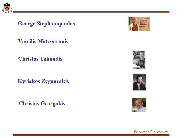George Stephanopoulos Vassilis Matzouranis Christos Takoudis Kyriakos Zygourakis Christos Georgakis Princeton University

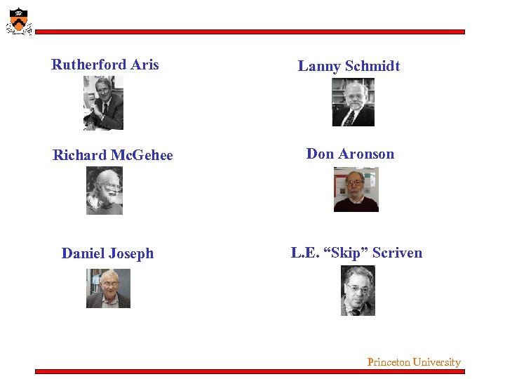Rutherford Aris Richard Mc. Gehee Daniel Joseph Lanny Schmidt Don Aronson L. E. “Skip” Scriven Princeton University

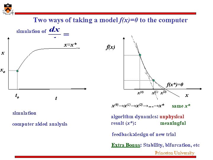Two ways of taking a model f(x)=0 to the computer simulation of x=x* x f(x) xo f(x*)=0 to t x(0) x(1) x(2) x(0)→x(1)→x(2)→…→x* simulation computer aided analysis x same x* algorithm dynamics: unphysical result (x*): meaningful feedback: design of new trial Extra Bonus: Stability, bifurcation, etc Princeton University

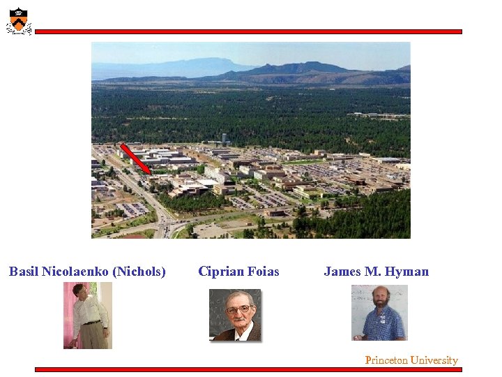Basil Nicolaenko (Nichols) Ciprian Foias James M. Hyman Princeton University

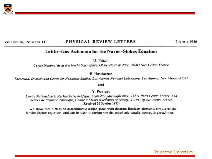Princeton University

Princeton University

Princeton University

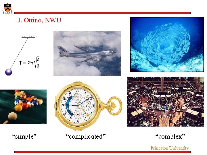J. Ottino, NWU “simple” “complicated” “complex” Princeton University

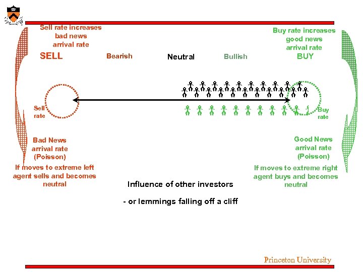Sell rate increases bad news arrival rate SELL Buy rate increases good news arrival rate Bearish Neutral Bad News Arrives No news – drift to Center jump left - Sell rate -1 Bad News arrival rate (Poisson) If moves to extreme left agent sells and becomes neutral BUY Bullish Good News Arrives jump right + 0 1 Buy rate Good News arrival rate (Poisson) Influence of other investors If moves to extreme right agent buys and becomes neutral - or lemmings falling off a cliff Princeton University

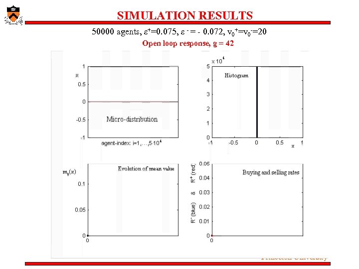SIMULATION RESULTS 50000 agents, ε+=0. 075, ε - = - 0. 072, v 0+=v 0 -=20 Open loop response, g = 42 Princeton University

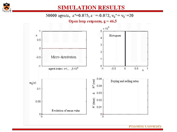SIMULATION RESULTS 50000 agents, ε+=0. 075, ε - =-0. 072, v 0+ = v 0 - =20 Open loop response, g = 46. 5 Princeton University

Multiscale / Complex System Modeling “Textbook” engineering modeling: macroscopic behavior through macroscopic models (e. g. conservation equations augmented by closures) Alternative (and increasingly frequent) modeling situation: • Models – at a FINE / ATOMISTIC / STOCHASTIC level – MD, KMC, BD, LB (also CPMD…) • Desired Behavior – At a COARSER, Macroscopic Level – E. g. Conservation equations, flow, reaction-diffusion, elasticity • Seek a bridge – Between Microscopic/Stochastic Simulation – And “Traditional, Continuum” Numerical Analysis – When closed macroscopic equations are not available in closed form Princeton University

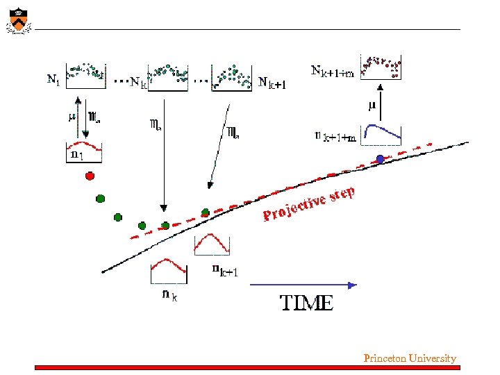
What I told you: Solve the equations WITHOUT writing them down. Write “software wrappers” around “fine level” microscopic codes Top level: all algorithms we know and love Bottom level: MD, k. MC, LB, BD, heterogeneous/ discrete media, CPMD, hybrid INTERFACE: Trade Function/Jacobian Evaluation for “on demand” experimentation and estimation Think of the microscopic simulator AS AN EXPERIMENT That you can set up and run at will “Equation Free” (motivated by “matrix free iterative linear algebra”) “Variable Free” (use of diffusion maps to discover good reduction coordinates) Princeton University

Princeton University

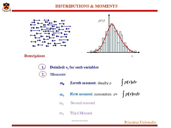DISTRIBUTIONS & MOMENTS p(v) Descriptions v 1. Detailed: vi for each variables 2. Moments m 0 Zeroth moment: density ρ m 1 First moment: momentum ρv m 2 Second moment m 3 Third Moment …………. Princeton University

Princeton University