e8986c8cb38f44853368c6451337796e.ppt
- Количество слайдов: 57
Advances in Pattern Databases Ariel Felner, Ben-Gurion University Israel email: felner@bgu. ac. il 1
Overview • • • Heuristic search and pattern databases Disjoint pattern databases Compressed pattern databases Dual lookups in pattern databases Current and future work 2
optimal path search algorithms • For small graphs: provided explicitly, algorithm such as Dijkstra’s shortest path, Bellman-Ford or Floyd-Warshal. Complexity O(n^2). • For very large graphs , which are implicitly defined, the A* algorithm which is a best-first search algorithm. 3
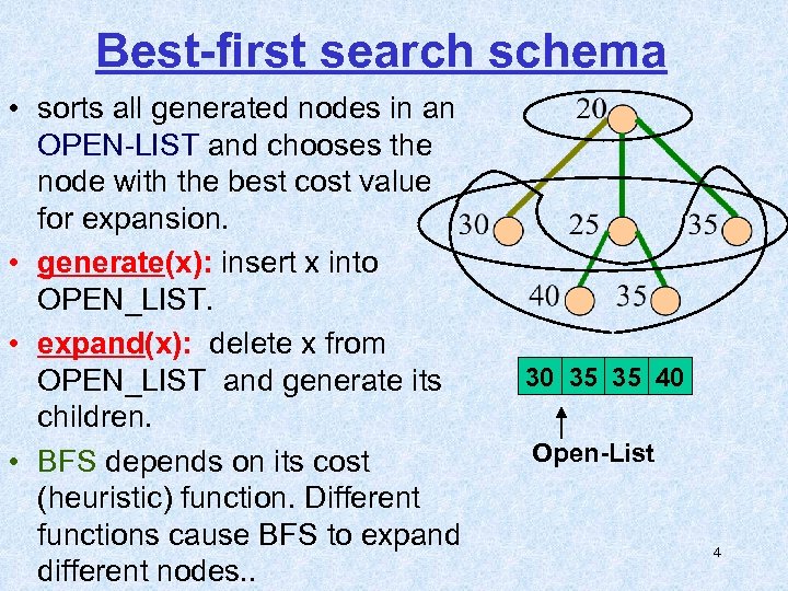
Best-first search schema • sorts all generated nodes in an OPEN-LIST and chooses the node with the best cost value for expansion. • generate(x): insert x into OPEN_LIST. • expand(x): delete x from OPEN_LIST and generate its children. • BFS depends on its cost (heuristic) function. Different functions cause BFS to expand different nodes. . 30 25 35 20 30 35 40 Open-List 4
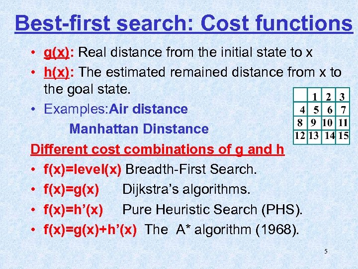
Best-first search: Cost functions • g(x): Real distance from the initial state to x • h(x): The estimated remained distance from x to the goal state. • Examples: Air distance Manhattan Dinstance Different cost combinations of g and h • f(x)=level(x) Breadth-First Search. • f(x)=g(x) Dijkstra’s algorithms. • f(x)=h’(x) Pure Heuristic Search (PHS). • f(x)=g(x)+h’(x) The A* algorithm (1968). 5
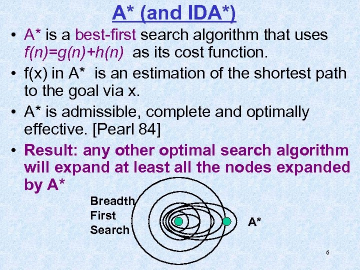
A* (and IDA*) • A* is a best-first search algorithm that uses f(n)=g(n)+h(n) as its cost function. • f(x) in A* is an estimation of the shortest path to the goal via x. • A* is admissible, complete and optimally effective. [Pearl 84] • Result: any other optimal search algorithm will expand at least all the nodes expanded by A* Breadth First Search A* 6
![Domains • • • 15 puzzle 10^13 states First solved by [Korf 85] with Domains • • • 15 puzzle 10^13 states First solved by [Korf 85] with](https://present5.com/presentation/e8986c8cb38f44853368c6451337796e/image-7.jpg)
Domains • • • 15 puzzle 10^13 states First solved by [Korf 85] with IDA* and Manhattan distance Takes 53 seconds 24 puzzle 10^24 states First solved by [Korf 96] Takes 2 days 7
![Domains • • Rubik’s cube 10^19 states First solved by [Korf 97] Takes 2 Domains • • Rubik’s cube 10^19 states First solved by [Korf 97] Takes 2](https://present5.com/presentation/e8986c8cb38f44853368c6451337796e/image-8.jpg)
Domains • • Rubik’s cube 10^19 states First solved by [Korf 97] Takes 2 days to solve 8
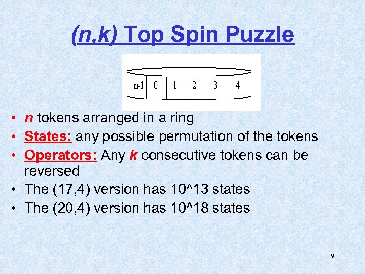
(n, k) Top Spin Puzzle • n tokens arranged in a ring • States: any possible permutation of the tokens • Operators: Any k consecutive tokens can be reversed • The (17, 4) version has 10^13 states • The (20, 4) version has 10^18 states 9
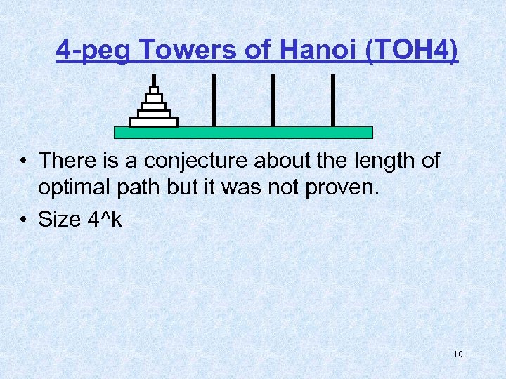
4 -peg Towers of Hanoi (TOH 4) • There is a conjecture about the length of optimal path but it was not proven. • Size 4^k 10
![How to improve search? • • • Enhanced algorithms: Perimeter-search [Delinberg and Nilson 95] How to improve search? • • • Enhanced algorithms: Perimeter-search [Delinberg and Nilson 95]](https://present5.com/presentation/e8986c8cb38f44853368c6451337796e/image-11.jpg)
How to improve search? • • • Enhanced algorithms: Perimeter-search [Delinberg and Nilson 95] RBFS [Korf 93] Frontier-search [Korf and Zang 2003] Breadth-first heuristic search [Zhou and Hansen 04] They all try to better explore the search tree. • Better heuristics: more parts of the search tree will be pruned. 11
Better heuristics • In the 3 rd Millennium we have very large memories. We can build large tables. • For enhanced algorithms: large open-lists or transposition tables. They store nodes explicitly. • A more intelligent way is to store general knowledge. We can do this with heuristics 12
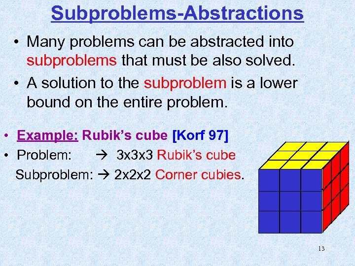
Subproblems-Abstractions • Many problems can be abstracted into subproblems that must be also solved. • A solution to the subproblem is a lower bound on the entire problem. • Example: Rubik’s cube [Korf 97] • Problem: 3 x 3 x 3 Rubik’s cube Subproblem: 2 x 2 x 2 Corner cubies. 13
![Pattern Databases heuristics • A pattern database [Culbreson & Schaeffer 96] is a lookup Pattern Databases heuristics • A pattern database [Culbreson & Schaeffer 96] is a lookup](https://present5.com/presentation/e8986c8cb38f44853368c6451337796e/image-14.jpg)
Pattern Databases heuristics • A pattern database [Culbreson & Schaeffer 96] is a lookup table that stores solutions to all configurations of the subproblem / abstraction / pattern. • This table is used as a heuristic during the search. • Example: Rubik’s cube. • Has 10^19 States. • The corner cubies subproblem has 88 Million states • A table with 88 Million entries fits in memory [Korf 97]. Search space Mapping/Projection Pattern space 14
![Non-additive pattern databases • Fringe pattern database [Culberson & Schaeffer 1996]. • Has only Non-additive pattern databases • Fringe pattern database [Culberson & Schaeffer 1996]. • Has only](https://present5.com/presentation/e8986c8cb38f44853368c6451337796e/image-15.jpg)
Non-additive pattern databases • Fringe pattern database [Culberson & Schaeffer 1996]. • Has only 259 Million states. • Improvement of a factor of 100 over Manhattan Distance 15
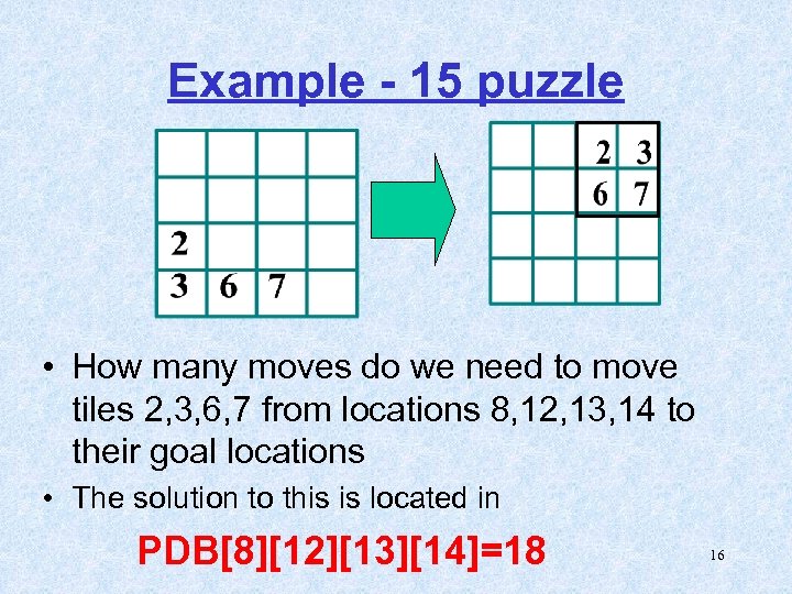
Example - 15 puzzle • How many moves do we need to move tiles 2, 3, 6, 7 from locations 8, 12, 13, 14 to their goal locations • The solution to this is located in PDB[8][12][13][14]=18 16
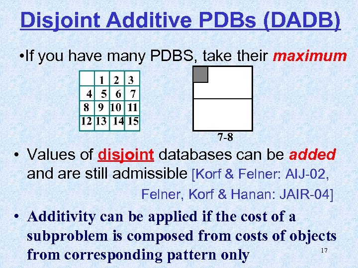
Disjoint Additive PDBs (DADB) • If you have many PDBS, take their maximum 7 -8 • Values of disjoint databases can be added and are still admissible [Korf & Felner: AIJ-02, Felner, Korf & Hanan: JAIR-04] • Additivity can be applied if the cost of a subproblem is composed from costs of objects 17 from corresponding pattern only
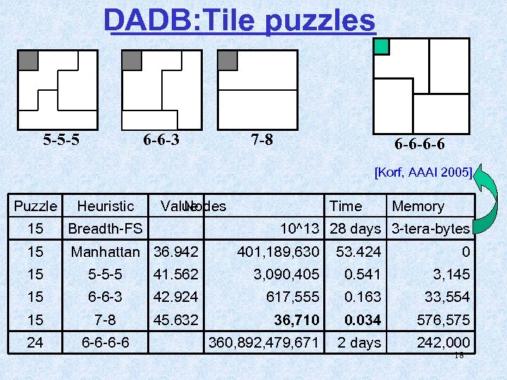
DADB: Tile puzzles 5 -5 -5 6 -6 -3 7 -8 6 -6 -6 -6 [Korf, AAAI 2005] Puzzle Heuristic Value Nodes 15 Breadth-FS 15 Manhattan 36. 942 Time Memory 10^13 28 days 3 -tera-bytes 401, 189, 630 53. 424 0 15 5 -5 -5 41. 562 3, 090, 405 0. 541 3, 145 15 6 -6 -3 42. 924 617, 555 0. 163 33, 554 15 7 -8 45. 632 36, 710 0. 034 576, 575 24 6 -6 -6 -6 360, 892, 479, 671 2 days 242, 000 18
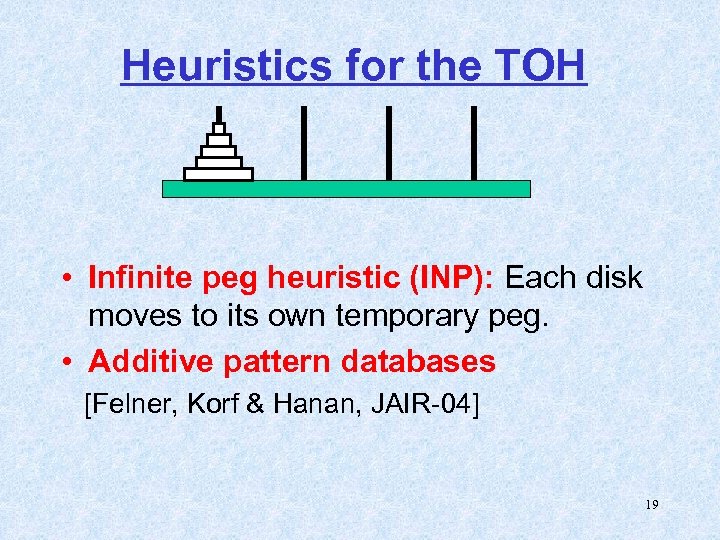
Heuristics for the TOH • Infinite peg heuristic (INP): Each disk moves to its own temporary peg. • Additive pattern databases [Felner, Korf & Hanan, JAIR-04] 19
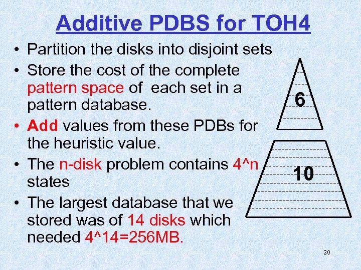
Additive PDBS for TOH 4 • Partition the disks into disjoint sets • Store the cost of the complete pattern space of each set in a pattern database. • Add values from these PDBs for the heuristic value. • The n-disk problem contains 4^n states • The largest database that we stored was of 14 disks which needed 4^14=256 MB. 6 10 20
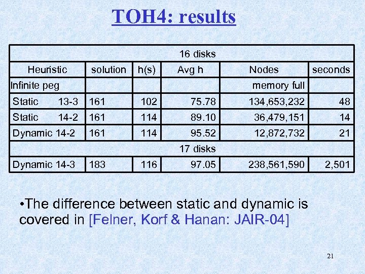
TOH 4: results 16 disks Heuristic solution h(s) Avg h Infinite peg Nodes seconds memory full Static 13 -3 161 102 75. 78 134, 653, 232 48 Static 14 -2 161 114 89. 10 36, 479, 151 14 Dynamic 14 -2 161 114 95. 52 12, 872, 732 21 238, 561, 590 2, 501 17 disks Dynamic 14 -3 183 116 97. 05 • The difference between static and dynamic is covered in [Felner, Korf & Hanan: JAIR-04] 21
Best Usage of Memory • Given 1 giga byte of memory, how do we best use it with pattern databases? • [Holte, Newton, Felner, Meshulam and Furcy, ICAPS-2004] showed that it is better to use many small databases and take their maximum instead of one large database. • We will present a different (orthogonal) method [Felner, Mushlam & Holte: AAAI-04]. 22
![Compressing pattern database [Felner et al AAAI-04] • Traditionally, each configuration of the pattern Compressing pattern database [Felner et al AAAI-04] • Traditionally, each configuration of the pattern](https://present5.com/presentation/e8986c8cb38f44853368c6451337796e/image-23.jpg)
Compressing pattern database [Felner et al AAAI-04] • Traditionally, each configuration of the pattern had a unique entry in the PDB. • Our main claim Nearby entries in PDBs are highly correlated !! • We propose to compress nearby entries by storing their minimum in one entry. • We show that most of the knowledge is preserved • Consequences: Memory is saved, larger patterns can be used speedup in search is obtained. 23
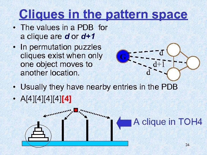
Cliques in the pattern space • The values in a PDB for a clique are d or d+1 • In permutation puzzles cliques exist when only one object moves to another location. G d d d+1 • Usually they have nearby entries in the PDB • A[4][4][4] A clique in TOH 4 24
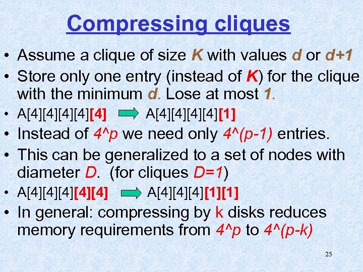
Compressing cliques • Assume a clique of size K with values d or d+1 • Store only one entry (instead of K) for the clique with the minimum d. Lose at most 1. • A[4][4][4] A[4][4][1] • Instead of 4^p we need only 4^(p-1) entries. • This can be generalized to a set of nodes with diameter D. (for cliques D=1) • A[4][4][4][1][1] • In general: compressing by k disks reduces memory requirements from 4^p to 4^(p-k) 25
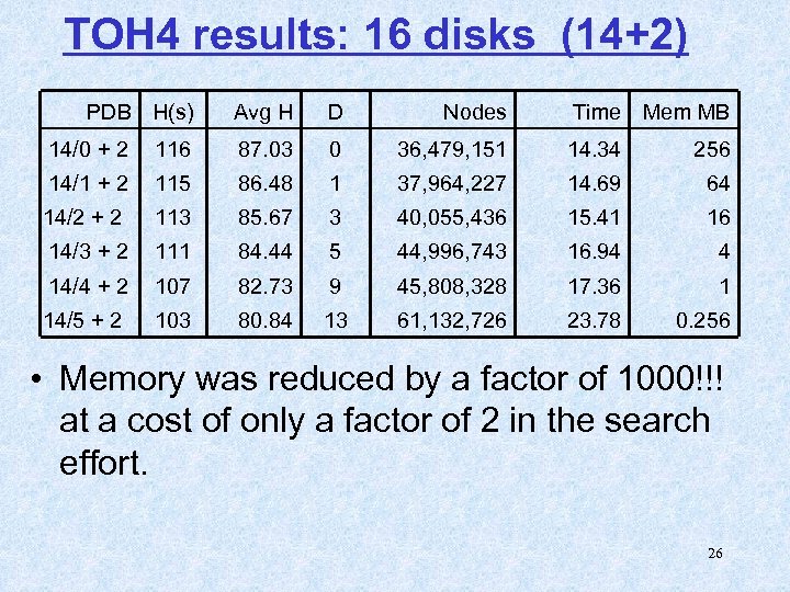
TOH 4 results: 16 disks (14+2) PDB H(s) Avg H D Nodes Time Mem MB 14/0 + 2 116 87. 03 0 36, 479, 151 14. 34 256 14/1 + 2 115 86. 48 1 37, 964, 227 14. 69 64 14/2 + 2 113 85. 67 3 40, 055, 436 15. 41 16 14/3 + 2 111 84. 44 5 44, 996, 743 16. 94 4 14/4 + 2 107 82. 73 9 45, 808, 328 17. 36 1 14/5 + 2 103 80. 84 13 61, 132, 726 23. 78 0. 256 • Memory was reduced by a factor of 1000!!! at a cost of only a factor of 2 in the search effort. 26
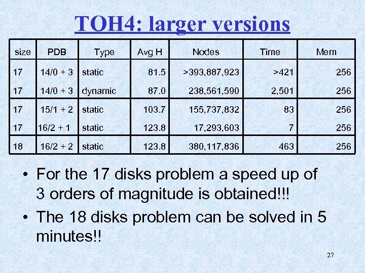
TOH 4: larger versions size PDB Type Avg H Nodes Time Mem 17 14/0 + 3 static 81. 5 >393, 887, 923 >421 256 17 14/0 + 3 dynamic 87. 0 238, 561, 590 2, 501 256 17 15/1 + 2 static 103. 7 155, 737, 832 83 256 17 16/2 + 1 static 123. 8 17, 293, 603 7 256 18 16/2 + 2 static 123. 8 380, 117, 836 463 256 • For the 17 disks problem a speed up of 3 orders of magnitude is obtained!!! • The 18 disks problem can be solved in 5 minutes!! 27
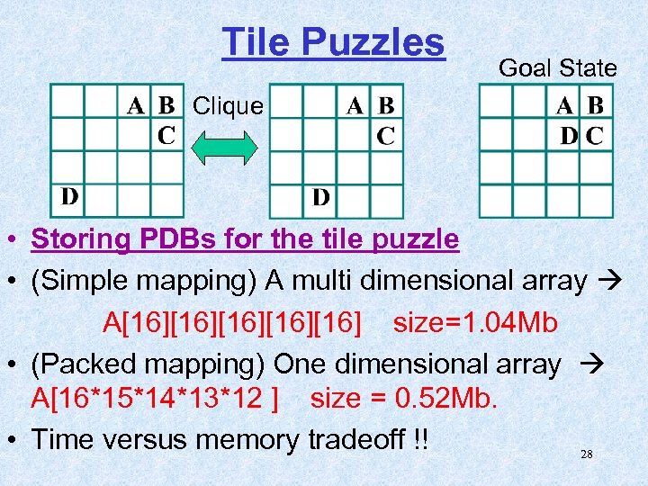
Tile Puzzles Goal State Clique • Storing PDBs for the tile puzzle • (Simple mapping) A multi dimensional array A[16][16][16] size=1. 04 Mb • (Packed mapping) One dimensional array A[16*15*14*13*12 ] size = 0. 52 Mb. • Time versus memory tradeoff !! 28
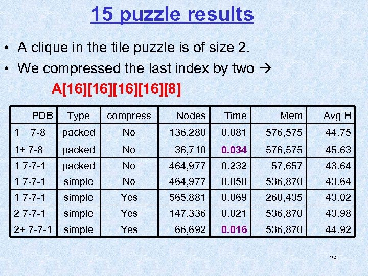
15 puzzle results • A clique in the tile puzzle is of size 2. • We compressed the last index by two A[16][16][8] PDB Type compress Nodes Time Mem Avg H 7 -8 packed No 136, 288 0. 081 576, 575 44. 75 1+ 7 -8 packed No 36, 710 0. 034 576, 575 45. 63 1 7 -7 -1 packed No 464, 977 0. 232 57, 657 43. 64 1 7 -7 -1 simple No 464, 977 0. 058 536, 870 43. 64 1 7 -7 -1 simple Yes 565, 881 0. 069 268, 435 43. 02 2 7 -7 -1 simple Yes 147, 336 0. 021 536, 870 43. 98 2+ 7 -7 -1 simple Yes 66, 692 0. 016 536, 870 44. 92 1 29
![• Dual lookups in pattern databases [Felner et al, IJCAI-04] 30 • Dual lookups in pattern databases [Felner et al, IJCAI-04] 30](https://present5.com/presentation/e8986c8cb38f44853368c6451337796e/image-30.jpg)
• Dual lookups in pattern databases [Felner et al, IJCAI-04] 30
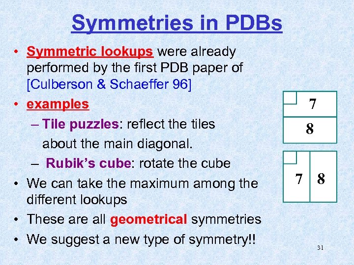
Symmetries in PDBs • Symmetric lookups were already performed by the first PDB paper of [Culberson & Schaeffer 96] • examples – Tile puzzles: reflect the tiles about the main diagonal. – Rubik’s cube: rotate the cube • We can take the maximum among the different lookups • These are all geometrical symmetries • We suggest a new type of symmetry!! 7 8 31
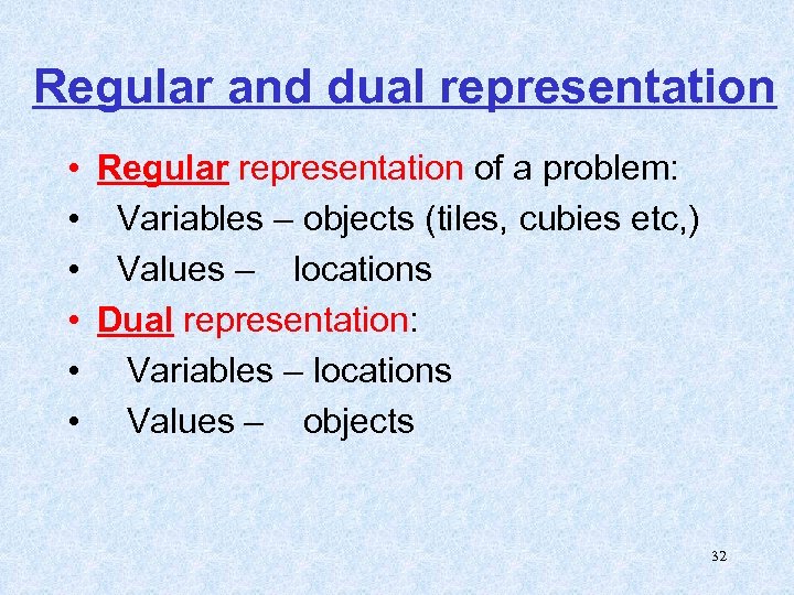
Regular and dual representation • Regular representation of a problem: • Variables – objects (tiles, cubies etc, ) • Values – locations • Dual representation: • Variables – locations • Values – objects 32
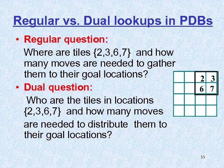
Regular vs. Dual lookups in PDBs • Regular question: Where are tiles {2, 3, 6, 7} and how many moves are needed to gather them to their goal locations? • Dual question: Who are the tiles in locations {2, 3, 6, 7} and how many moves are needed to distribute them to their goal locations? 33
![Regular and dual lookups • Regular lookup: PDB[8, 12, 13, 14] • Dual lookup: Regular and dual lookups • Regular lookup: PDB[8, 12, 13, 14] • Dual lookup:](https://present5.com/presentation/e8986c8cb38f44853368c6451337796e/image-34.jpg)
Regular and dual lookups • Regular lookup: PDB[8, 12, 13, 14] • Dual lookup: PDB[9, 5, 12, 15] 34
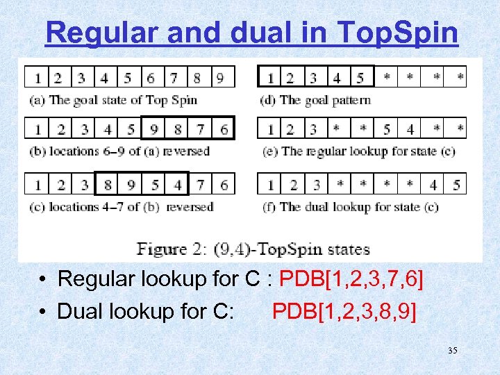
Regular and dual in Top. Spin • Regular lookup for C : PDB[1, 2, 3, 7, 6] • Dual lookup for C: PDB[1, 2, 3, 8, 9] 35
Dual lookups • Dual lookups are possible when there is a symmetry between locations and objects: – Each object is in only one location and each location occupies only one object. • Good examples: Top. Spin, Rubik’s cube • Bad example: Towers of Hanoi • Problematic example: Tile Puzzles 36
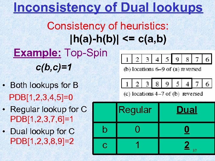
Inconsistency of Dual lookups Consistency of heuristics: |h(a)-h(b)| <= c(a, b) Example: Top-Spin c(b, c)=1 • Both lookups for B PDB[1, 2, 3, 4, 5]=0 • Regular lookup for C PDB[1, 2, 3, 7, 6]=1 • Dual lookup for C PDB[1, 2, 3, 8, 9]=2 Regular Dual b 0 0 c 1 2 37
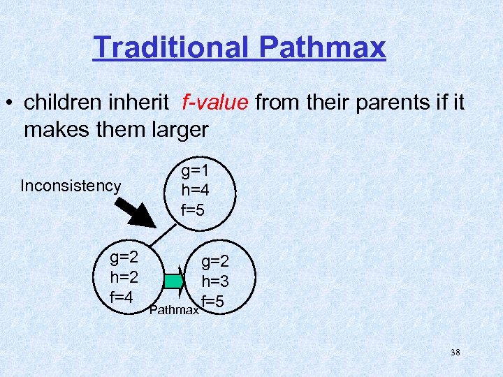
Traditional Pathmax • children inherit f-value from their parents if it makes them larger Inconsistency g=2 h=2 f=4 g=1 h=4 f=5 g=2 h=3 f=5 Pathmax 38
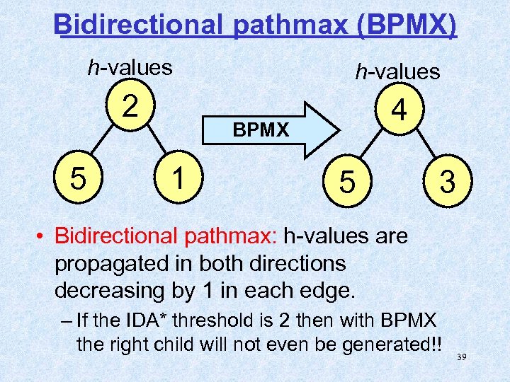
Bidirectional pathmax (BPMX) h-values 2 5 h-values 4 BPMX 1 5 3 • Bidirectional pathmax: h-values are propagated in both directions decreasing by 1 in each edge. – If the IDA* threshold is 2 then with BPMX the right child will not even be generated!! 39
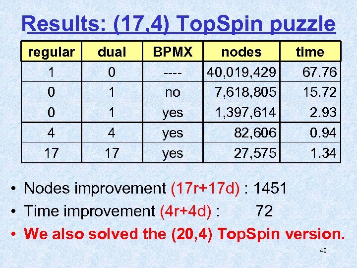
Results: (17, 4) Top. Spin puzzle regular 1 0 0 4 17 dual 0 1 1 4 17 BPMX ---no yes yes nodes 40, 019, 429 7, 618, 805 1, 397, 614 82, 606 27, 575 time 67. 76 15. 72 2. 93 0. 94 1. 34 • Nodes improvement (17 r+17 d) : 1451 • Time improvement (4 r+4 d) : 72 • We also solved the (20, 4) Top. Spin version. 40
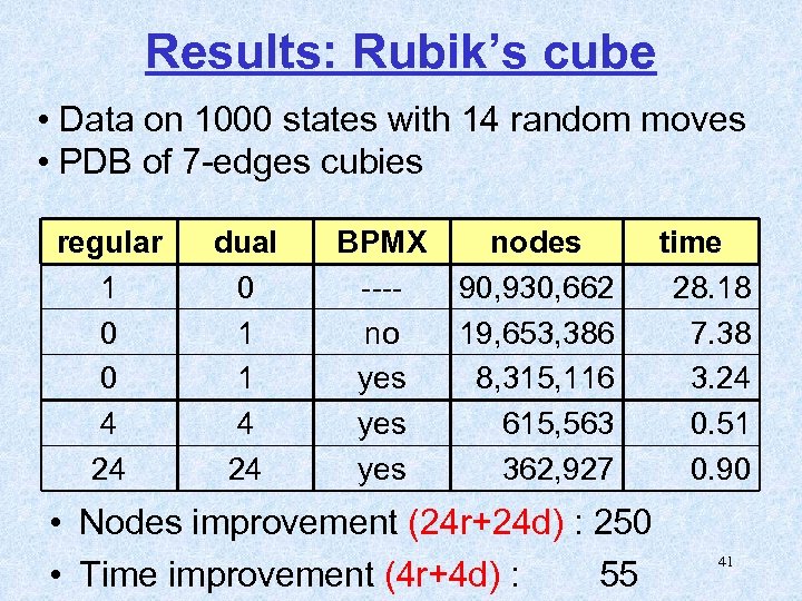
Results: Rubik’s cube • Data on 1000 states with 14 random moves • PDB of 7 -edges cubies regular 1 0 0 4 24 dual 0 1 1 4 24 BPMX ---no yes yes nodes 90, 930, 662 19, 653, 386 8, 315, 116 615, 563 362, 927 • Nodes improvement (24 r+24 d) : 250 • Time improvement (4 r+4 d) : 55 time 28. 18 7. 38 3. 24 0. 51 0. 90 41
Results: Rubik’s cube • With duals we improved Korf’s results on random instances by a factor of 1. 5 using exactly the same PDBs. 42
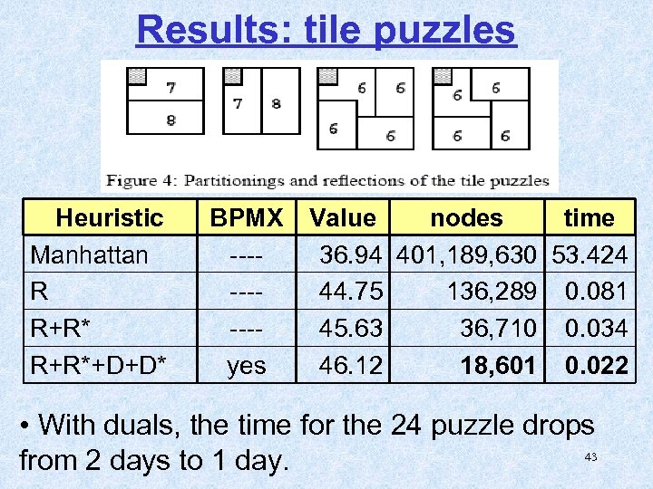
Results: tile puzzles Heuristic Manhattan R R+R*+D+D* BPMX -----yes Value nodes time 36. 94 401, 189, 630 53. 424 44. 75 136, 289 0. 081 45. 63 36, 710 0. 034 46. 12 18, 601 0. 022 • With duals, the time for the 24 puzzle drops 43 from 2 days to 1 day.
Discussion • Results for the Top. Spin and Rubik’s cube are better than those of the tile puzzles • Dual PDB lookups and BPMX cutoffs are more effective if each operators changes larger part of the states. • This is because the identity of the objects being queried in consecutive states are dramatically changed 44
Summary • Dual PDB lookups • BPMX cutoffs for inconsistent heuristics • State of the art solvers. 45
Future work • • • More compression Duality in search spaces Which and how many symmetries to use Other sources of inconsistencies Better ways for propagating inconsistencies 46
Ongoing and future work compressing PDBs • An item for the PDB of tiles (a, b, c, d) is in the form: <La, Lb, Lc, Ld>=d • Store the PDBs in a Trie • A PDB of 5 tiles will have a level in the trie for each tile. The values will be in the leaves of the trie. • This data-structure will enable flexibility and will save memory as subtrees of the trie can be pruned 47
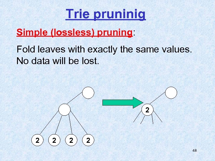
Trie pruninig Simple (lossless) pruning: Fold leaves with exactly the same values. No data will be lost. 2 2 2 48
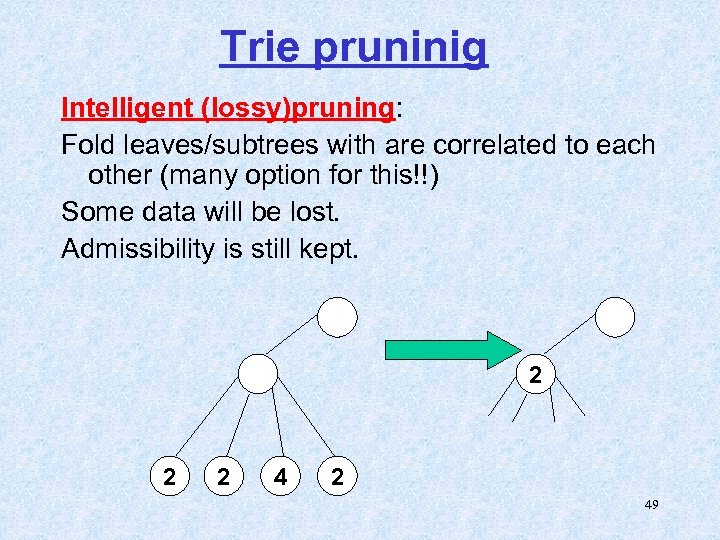
Trie pruninig Intelligent (lossy)pruning: Fold leaves/subtrees with are correlated to each other (many option for this!!) Some data will be lost. Admissibility is still kept. 2 2 2 49
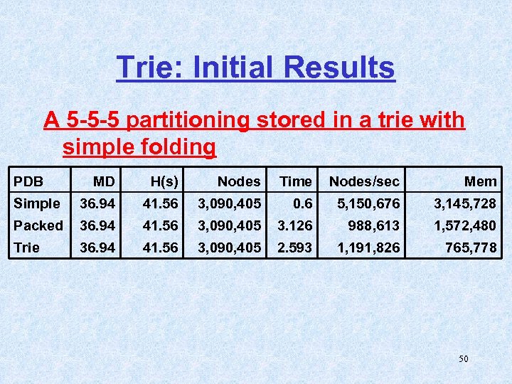
Trie: Initial Results A 5 -5 -5 partitioning stored in a trie with simple folding PDB MD H(s) Nodes Time Nodes/sec Mem Simple 36. 94 41. 56 3, 090, 405 0. 6 5, 150, 676 3, 145, 728 Packed 36. 94 41. 56 3, 090, 405 3. 126 988, 613 1, 572, 480 Trie 36. 94 41. 56 3, 090, 405 2. 593 1, 191, 826 765, 778 50
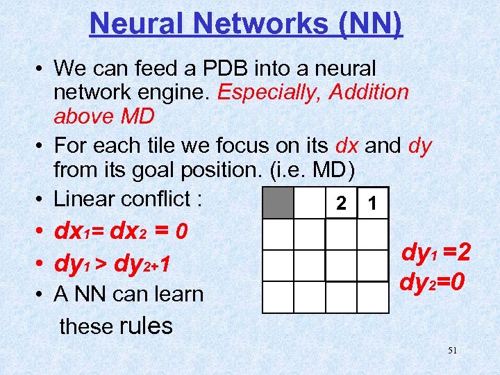
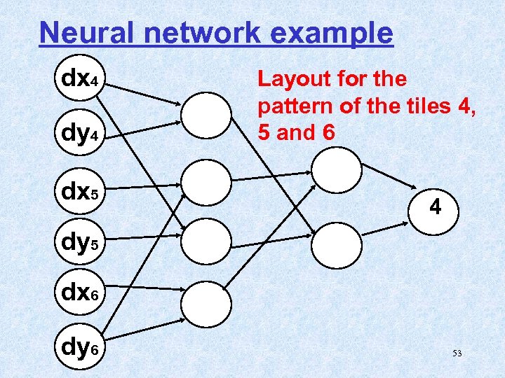
Neural Networks (NN) • We can feed a PDB into a neural network engine. Especially, Addition above MD • For each tile we focus on its dx and dy from its goal position. (i. e. MD) • Linear conflict : 2 1 • dx 1= dx 2 = 0 dy 1 =2 • dy 1 > dy 2+1 dy 2=0 • A NN can learn these rules 51
Neural network • We train the NN by feeding the entire (or part of the) pattern space. • For example for a pattern of 5 tiles we have 10 features, 2 for each tile. • During the search, given the locations of the tiles we look them up in the NN. 52
Neural network example dx 4 dy 4 dx 5 Layout for the pattern of the tiles 4, 5 and 6 4 dy 5 dx 6 dy 6 53
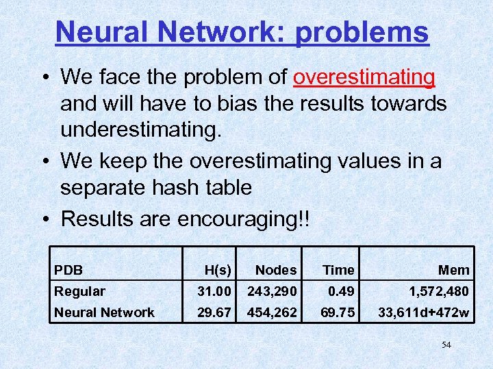
Neural Network: problems • We face the problem of overestimating and will have to bias the results towards underestimating. • We keep the overestimating values in a separate hash table • Results are encouraging!! PDB H(s) Nodes Time Mem Regular 31. 00 243, 290 0. 49 1, 572, 480 Neural Network 29. 67 454, 262 69. 75 33, 611 d+472 w 54
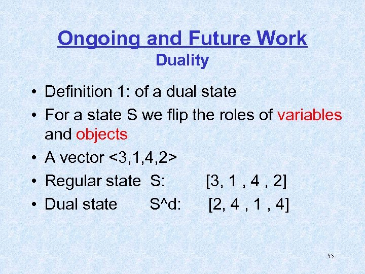
Ongoing and Future Work Duality • Definition 1: of a dual state • For a state S we flip the roles of variables and objects • A vector <3, 1, 4, 2> • Regular state S: [3, 1 , 4 , 2] • Dual state S^d: [2, 4 , 1 , 4] 55
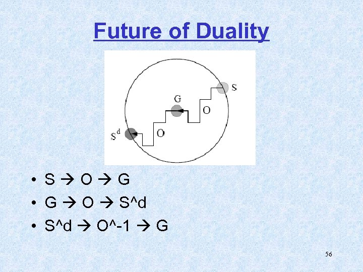
Future of Duality • S O G • G O S^d • S^d O^-1 G 56
Workshop You are all welcome to the workshop on: ”Heuristic Search, Memory-based Heuristics and Their application” To be held in AAAI-06 See: www. ise. bgu. ac. il/faculty/felner 57
e8986c8cb38f44853368c6451337796e.ppt