Advanced Algorithms Piyush Kumar Lecture 17 Online Algorithms

Advanced Algorithms Piyush Kumar (Lecture 17: Online Algorithms) Welcome to COT 5405

On Bounds • Worst Case. • Average Case: Running time over some distribution of input. (Quicksort) • Amortized Analysis: Worst case bound on sequence of operations. – (Bit Increments, Union-Find) • Competitive Analysis: Compare the cost of an online algorithm with an optimal prescient algorithm on any sequence of requests. – Today.

Problem 1 • The online dating game. – You get to date fixed number of partners. – You either choose to pick them up or try your luck again. – You can not go back in time. – What strategy would you use to pick?

Problem 2. • You like to Ski. • When weather AND mood permits, you go skiing • If you own the equipment, you take it with you, Otherwise Rent. • You can buy the equipment whenever you decide, but not while skiing.

Costs • 1 Unit to rent, M units to buy • If you go ski I times, what is OPT? OPT = min (I, M) What algorithm should you use to decide whether you Should buy the equipment?

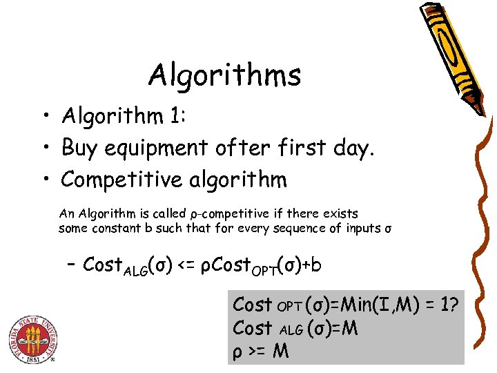Algorithms • Algorithm 1: • Buy equipment ofter first day. • Competitive algorithm An Algorithm is called ρ-competitive if there exists some constant b such that for every sequence of inputs σ – Cost. ALG(σ) <= ρCost. OPT(σ)+b Cost OPT (σ)=Min(I, M) = 1? Cost ALG (σ)=M ρ >= M

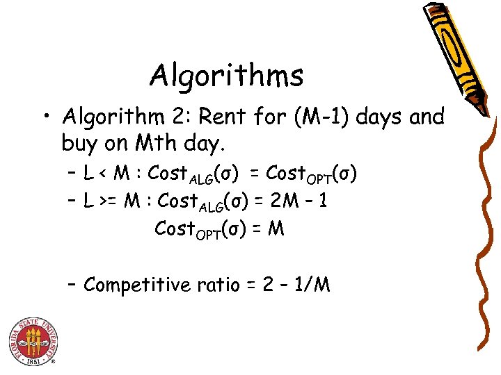Algorithms • Algorithm 2: Rent for (M-1) days and buy on Mth day. – L < M : Cost. ALG(σ) = Cost. OPT(σ) – L >= M : Cost. ALG(σ) = 2 M – 1 Cost. OPT(σ) = M – Competitive ratio = 2 – 1/M

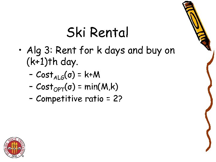Ski Rental • Alg 3: Rent for k days and buy on (k+1)th day. – Cost. ALG(σ) = k+M – Cost. OPT(σ) = min(M, k) – Competitive ratio = 2?

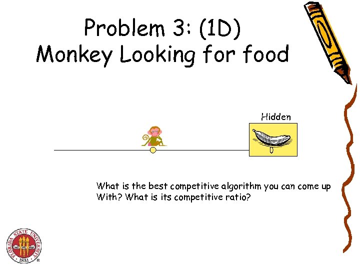Problem 3: (1 D) Monkey Looking for food Hidden What is the best competitive algorithm you can come up With? What is its competitive ratio?

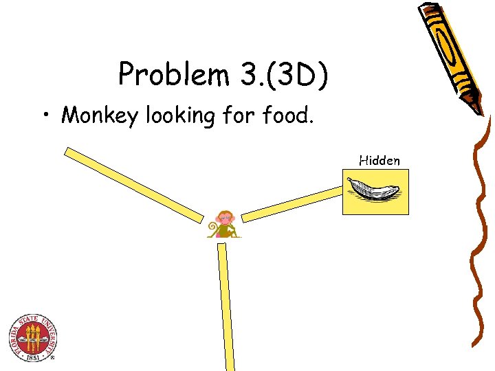Problem 3. (3 D) • Monkey looking for food. Hidden

On Line Algorithms • Work without full knowledge of the future • Deal with a sequence of events • Future events are unknown to the algorithm • The algorithm has to deal with one event at each time. The next event happens only after the algorithm is done dealing with the previous event

On-Line versus off-line • We compare the behavior of the online algorithm to an optimal off-line algorithm “OPT” which is familiar with the sequence • The off-line algorithm knows the exact properties of all the events in the sequence

Absolute competitive ratio (for minimization problems) • We measure the performance of an on-line algorithm by the competitive ratio • This is the ratio between what the on-line algorithms “pays” to what the optimal off-line algorithm “pays”

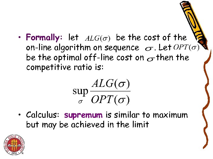• Formally: let be the cost of the on-line algorithm on sequence. Let be the optimal off-line cost on the competitive ratio is: • Calculus: supremum is similar to maximum but may be achieved in the limit

Problem 4: Caching • K-competitive caching. • Two level memory model • If a page is not in the cache , a page fault occurs. • A Paging algorithm specifies which page to evict on a fault. • Paging algorithms are online algorithms for cache replacement.

Online Paging Algorithms • Assumption: cache can hold k-pages. • CPU accesses memory thru cache. • Each request specifies a page in the memory system. – We want to minimize the page faults.

A Lower bound • Theorem: Let A be a deterministic online paging algorithm. If A is -competitive, then k. • Pf: Let S ={p_1, p_2, … , p_k+1} be a set of k+1 arbitrary memory pages. Assume w. l. g. that A and OPT initially have p_1, … , p_k in their cache. In the worst case A has a page fault on any request t.

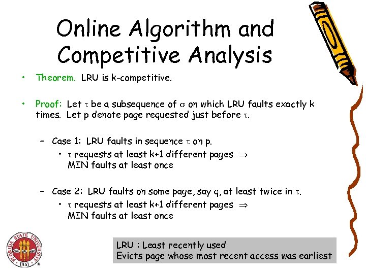Online Algorithm and Competitive Analysis • Theorem. LRU is k-competitive. • Proof: Let be a subsequence of on which LRU faults exactly k times. Let p denote page requested just before . – Case 1: LRU faults in sequence on p. • requests at least k+1 different pages MIN faults at least once – Case 2: LRU faults on some page, say q, at least twice in . • requests at least k+1 different pages MIN faults at least once LRU : Least recently used Evicts page whose most recent access was earliest

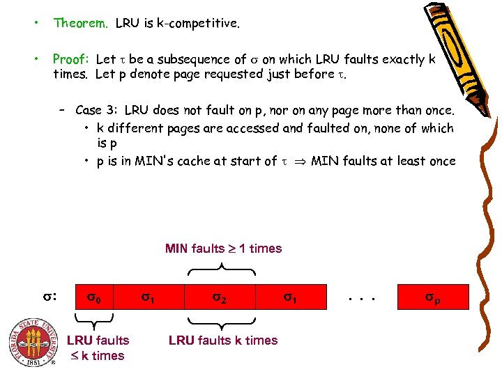• Theorem. LRU is k-competitive. • Proof: Let be a subsequence of on which LRU faults exactly k times. Let p denote page requested just before . – Case 3: LRU does not fault on p, nor on any page more than once. • k different pages are accessed and faulted on, none of which is p • p is in MIN's cache at start of MIN faults at least once MIN faults 1 times : 0 LRU faults k times 1 2 LRU faults k times 1 . . . p

Universal Hashing

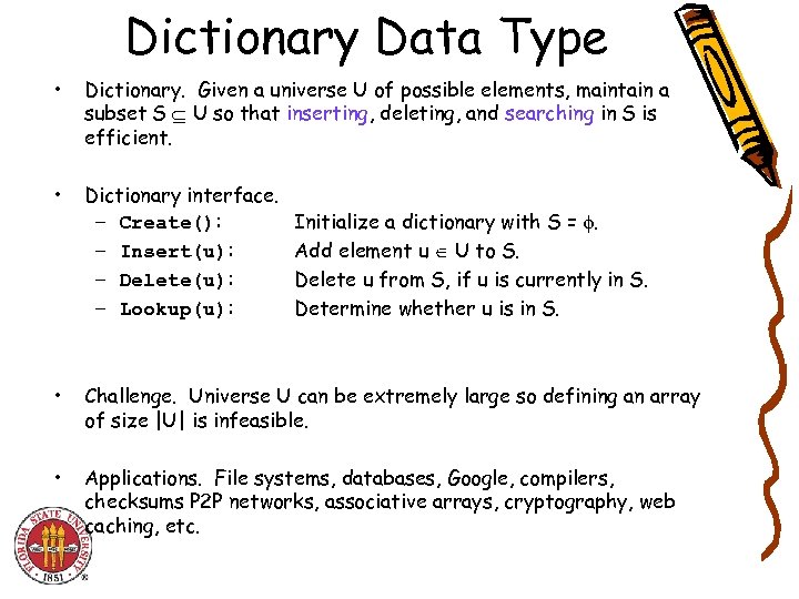Dictionary Data Type • Dictionary. Given a universe U of possible elements, maintain a subset S U so that inserting, deleting, and searching in S is efficient. • Dictionary interface. – Create(): – Insert(u): – Delete(u): – Lookup(u): • Challenge. Universe U can be extremely large so defining an array of size |U| is infeasible. • Applications. File systems, databases, Google, compilers, checksums P 2 P networks, associative arrays, cryptography, web caching, etc. Initialize a dictionary with S = . Add element u U to S. Delete u from S, if u is currently in S. Determine whether u is in S.

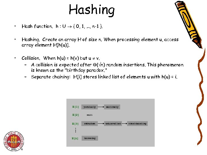Hashing • Hash function. h : U { 0, 1, …, n-1 }. • Hashing. Create an array H of size n. When processing element u, access array element H[h(u)]. • Collision. When h(u) = h(v) but u v. – A collision is expected after ( n) random insertions. This phenomenon is known as the "birthday paradox. " – Separate chaining: H[i] stores linked list of elements u with h(u) = i. H[1] jocularly H[2] null H[3] suburban H[n] browsing seriously untravelled considerating

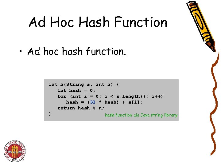Ad Hoc Hash Function • Ad hoc hash function. int h(String s, int n) { int hash = 0; for (int i = 0; i < s. length(); i++) hash = (31 * hash) + s[i]; return hash % n; } hash function ala Java string library

Algorithmic Complexity Attacks • When can't we live with ad hoc hash function? – Obvious situations: aircraft control, nuclear reactors. – Surprising situations: denial-of-service attacks. malicious adversary learns your ad hoc hash function (e. g. , by reading Java API) and causes a big pile-up in a single slot that grinds performance to a halt • Real world exploits. [Crosby-Wallach 2003] – Bro server: send carefully chosen packets to DOS the server, using less bandwidth than a dial-up modem – Perl 5. 8. 0: insert carefully chosen strings into associative array. – Linux 2. 4. 20 kernel: save files with carefully chosen names.

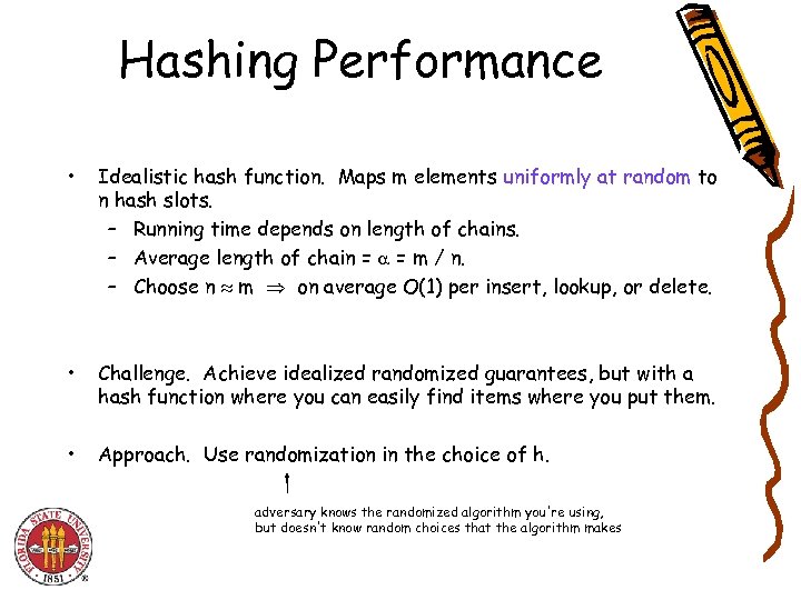Hashing Performance • Idealistic hash function. Maps m elements uniformly at random to n hash slots. – Running time depends on length of chains. – Average length of chain = = m / n. – Choose n m on average O(1) per insert, lookup, or delete. • Challenge. Achieve idealized randomized guarantees, but with a hash function where you can easily find items where you put them. • Approach. Use randomization in the choice of h. adversary knows the randomized algorithm you're using, but doesn't know random choices that the algorithm makes

Universal Hashing • Universal class of hash functions. [Carter-Wegman 1980 s] – For any pair of elements u, v U, – Can select random h efficiently. chosen uniformly at random – Can compute h(u) efficiently. • Ex. U = { a, b, c, d, e, f }, n = 2. a b c d e f h 1(x) 0 1 0 1 0 1 h 2(x) 0 0 0 1 1 1 h 3(x) 0 0 1 1 h 4(x) 1 0 0 1 1 0 H = {h 1, h 2} Pr h H [h(a) = h(b)] = 1/2 Pr h H [h(a) = h(c)] = 1 Pr h H [h(a) = h(d)] = 0. . . H = {h 1, h 2 , h 3 , h 4} Pr h H [h(a) = h(b)] Pr h H [h(a) = h(c)] Pr h H [h(a) = h(d)] Pr h H [h(a) = h(e)] Pr h H [h(a) = h(f)]. . . = = = 1/2 1/2 0 not universal

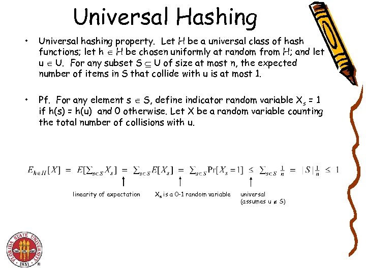Universal Hashing • Universal hashing property. Let H be a universal class of hash functions; let h H be chosen uniformly at random from H; and let u U. For any subset S U of size at most n, the expected number of items in S that collide with u is at most 1. • Pf. For any element s S, define indicator random variable Xs = 1 if h(s) = h(u) and 0 otherwise. Let X be a random variable counting the total number of collisions with u. linearity of expectation Xs is a 0 -1 random variable universal (assumes u S)

Designing a Universal Family of Hash Functions • Theorem. [Chebyshev 1850] There exists a prime between n and no need for randomness here 2 n. • Modulus. Choose a prime number p n. • Integer encoding. Identify each element u U with a base-p integer of r digits: x = (x 1, x 2, …, xr). • Hash function. Let A = set of all r-digit, base-p integers. For each a = (a 1, a 2, …, ar) where 0 ai < p, define • Hash function family. H = { ha : a A }.

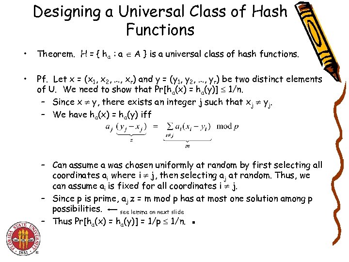Designing a Universal Class of Hash Functions • Theorem. H = { ha : a A } is a universal class of hash functions. • Pf. Let x = (x 1, x 2, …, xr) and y = (y 1, y 2, …, yr) be two distinct elements of U. We need to show that Pr[ha(x) = ha(y)] 1/n. – Since x y, there exists an integer j such that xj yj. – We have ha(x) = ha(y) iff – Can assume a was chosen uniformly at random by first selecting all coordinates ai where i j, then selecting aj at random. Thus, we can assume ai is fixed for all coordinates i j. – Since p is prime, aj z = m mod p has at most one solution among p possibilities. see lemma on next slide – Thus Pr[ha(x) = ha(y)] = 1/p 1/n. ▪

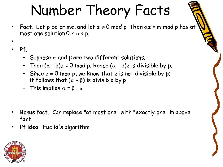Number Theory Facts • • • Fact. Let p be prime, and let z 0 mod p. Then z = m mod p has at most one solution 0 < p. Pf. – Suppose and are two different solutions. – Then ( - )z = 0 mod p; hence ( - )z is divisible by p. – Since z 0 mod p, we know that z is not divisible by p; it follows that ( - ) is divisible by p. – This implies = . ▪ Bonus fact. Can replace "at most one" with "exactly one" in above fact. Pf idea. Euclid's algorithm.