204fe27ab4a456856ecd1f7636d93bc4.ppt
- Количество слайдов: 17
Adding Support for Theory in Open Science Big Data John A. Miller, Hao Peng and Michael E. Cotterell Department of Computer Science University of Georgia Athens, GA, USA
Outline § Basic Definitions § Predictive Analytics § Using Theory in Model Development § Representing Theory
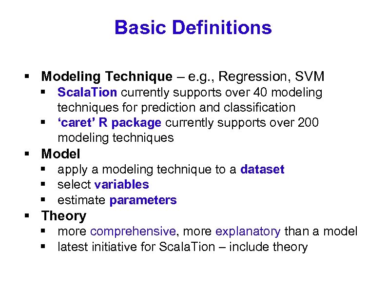
Basic Definitions § Modeling Technique – e. g. , Regression, SVM § Scala. Tion currently supports over 40 modeling techniques for prediction and classification § ‘caret’ R package currently supports over 200 modeling techniques § Model § apply a modeling technique to a dataset § select variables § estimate parameters § Theory § more comprehensive, more explanatory than a model § latest initiative for Scala. Tion – include theory
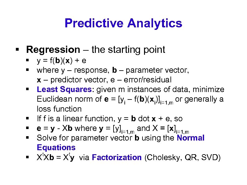
Predictive Analytics § Regression – the starting point § y = f(b)(x) + e § where y – response, b – parameter vector, x – predictor vector, e – error/residual § Least Squares: given m instances of data, minimize Euclidean norm of e = [yi – f(b)(xi)]i=1, m or generally a loss function § If f is a linear function, y = b dot x + e, so § e = y - Xb where y = [y]i=1, m and X = [x]i=1, m § Solve for parameter vector b using the Normal Equations § Xt. Xb = Xty via Factorization (Cholesky, QR, SVD)
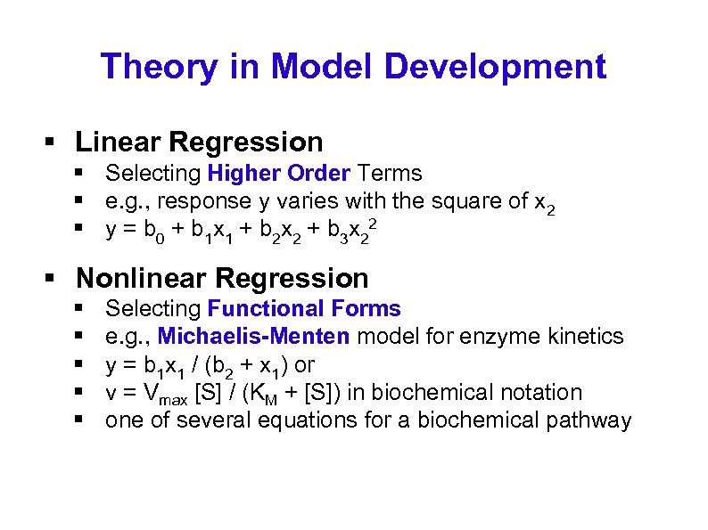
Theory in Model Development § Linear Regression § Selecting Higher Order Terms § e. g. , response y varies with the square of x 2 § y = b 0 + b 1 x 1 + b 2 x 2 + b 3 x 22 § Nonlinear Regression § § § Selecting Functional Forms e. g. , Michaelis-Menten model for enzyme kinetics y = b 1 x 1 / (b 2 + x 1) or v = Vmax [S] / (KM + [S]) in biochemical notation one of several equations for a biochemical pathway
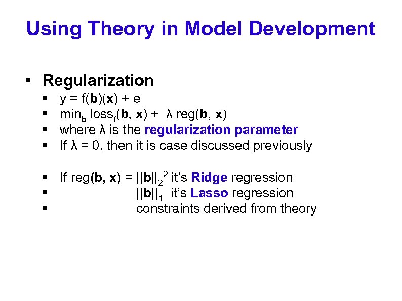
Using Theory in Model Development § Regularization § § y = f(b)(x) + e minb lossf(b, x) + λ reg(b, x) where λ is the regularization parameter If λ = 0, then it is case discussed previously § If reg(b, x) = ||b||22 it’s Ridge regression § ||b||1 it’s Lasso regression § constraints derived from theory
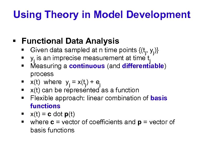
Using Theory in Model Development § Functional Data Analysis § Given data sampled at n time points {(tj, yj)} § yj is an imprecise measurement at time tj § Measuring a continuous (and differentiable) process § x(t) where yj = x(tj) + ej § x(t) can be represented as a function § Flexible approach: linear combination of basis functions § x(t) = c dot p(t) § where c = vector of coefficients and p = vector of basis functions
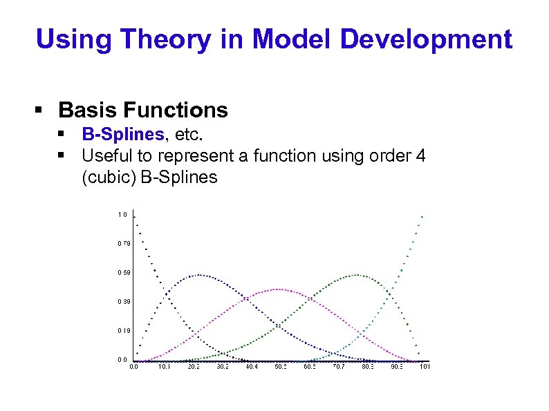
Using Theory in Model Development § Basis Functions § B-Splines, etc. § Useful to represent a function using order 4 (cubic) B-Splines
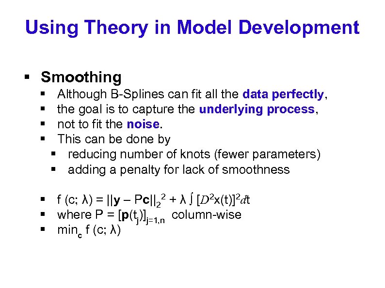
Using Theory in Model Development § Smoothing § § Although B-Splines can fit all the data perfectly, the goal is to capture the underlying process, not to fit the noise. This can be done by § reducing number of knots (fewer parameters) § adding a penalty for lack of smoothness § f (c; λ) = ||y – Pc||22 + λ ∫ [D 2 x(t)]2 dt § where P = [p(tj)]j=1, n column-wise § minc f (c; λ)
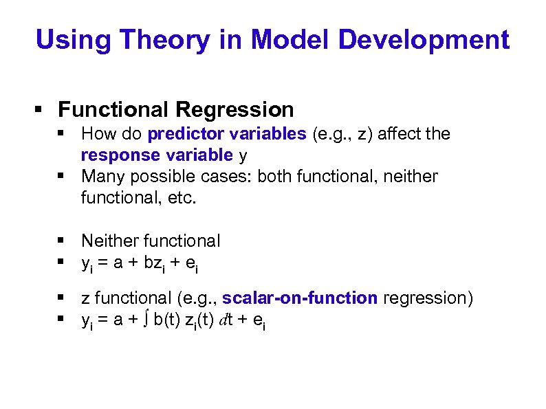
Using Theory in Model Development § Functional Regression § How do predictor variables (e. g. , z) affect the response variable y § Many possible cases: both functional, neither functional, etc. § Neither functional § yi = a + bzi + ei § z functional (e. g. , scalar-on-function regression) § yi = a + ∫ b(t) zi(t) dt + ei
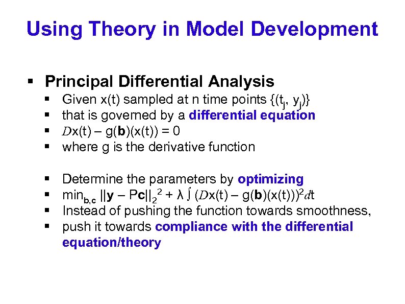
Using Theory in Model Development § Principal Differential Analysis § § Given x(t) sampled at n time points {(tj, yj)} that is governed by a differential equation Dx(t) – g(b)(x(t)) = 0 where g is the derivative function § § Determine the parameters by optimizing minb, c ||y – Pc||22 + λ ∫ (Dx(t) – g(b)(x(t)))2 dt Instead of pushing the function towards smoothness, push it towards compliance with the differential equation/theory
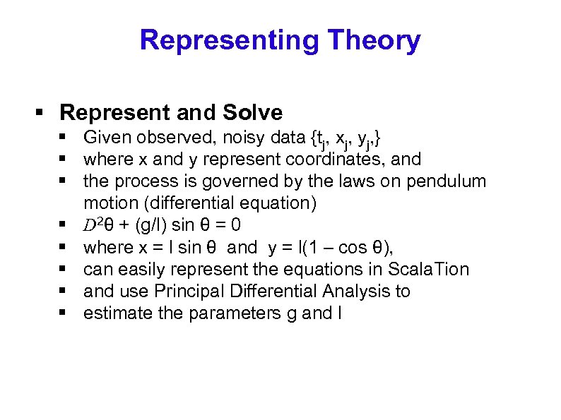
Representing Theory § Represent and Solve § Given observed, noisy data {tj, xj, yj, } § where x and y represent coordinates, and § the process is governed by the laws on pendulum motion (differential equation) § D 2θ + (g/l) sin θ = 0 § where x = l sin θ and y = l(1 – cos θ), § can easily represent the equations in Scala. Tion § and use Principal Differential Analysis to § estimate the parameters g and l
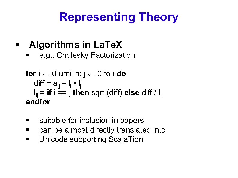
Representing Theory § Algorithms in La. Te. X § e. g. , Cholesky Factorization for i ← 0 until n; j ← 0 to i do diff = aij – li • lj lij = if i == j then sqrt (diff) else diff / ljj endfor § § § suitable for inclusion in papers can be almost directly translated into Unicode supporting Scala. Tion
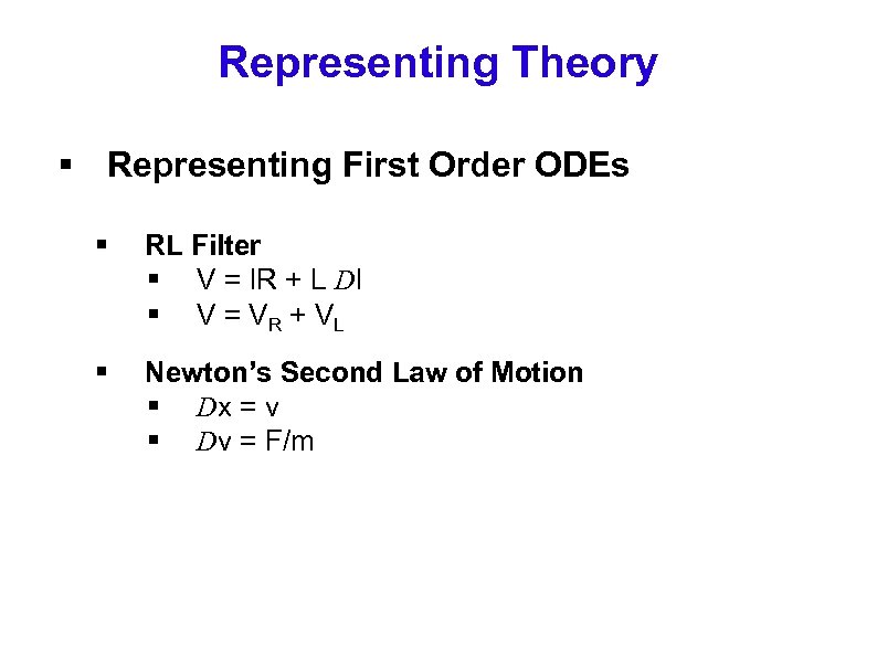
Representing Theory § Representing First Order ODEs § RL Filter § V = IR + L DI § V = VR + VL § Newton’s Second Law of Motion § Dx = v § Dv = F/m
![Representing Theory Chemical Reaction Network (www. cs. uga. edu/~thiab/paper 25. pdf) // d[H 2]/dt Representing Theory Chemical Reaction Network (www. cs. uga. edu/~thiab/paper 25. pdf) // d[H 2]/dt](https://present5.com/presentation/204fe27ab4a456856ecd1f7636d93bc4/image-15.jpg)
Representing Theory Chemical Reaction Network (www. cs. uga. edu/~thiab/paper 25. pdf) // d[H 2]/dt = - kf 1 [H 2] [O] + kb 1 [H] [OH] - kf 3 [H 2] [OH] + kb 3 [H 2 O] [H] def dh 2_dt (t: Double) = -kf. _1*c(0)*c(2) + kb. _1*c(3)*c(4) - kf. _3*c(0)*c(4) + kb. _3*c(5)*c(3) // d[O 2]/dt = - kf 2 [H] [O 2] + kb 2 [O] [OH] def do 2_dt (t: Double) = -kf. _2*c(3)*c(1) + kb. _2*c(2)*c(4) Two of eight ODEs in a common pathway. § Given rate constants kf and kb, use integrator to solve for concentrations c over time § Given time series data, estimate the rate constants using techniques discussed
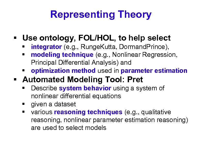
Representing Theory § Use ontology, FOL/HOL, to help select § integrator (e. g. , Runge. Kutta, Dormand. Prince), § modeling technique (e. g. , Nonlinear Regression, Principal Differential Analysis) and § optimization method used in parameter estimation § Automated Modeling Tool: Pret § Describe system behavior using a system of nonlinear differential equations § given a dataset § various reasoning techniques (e. g. , qualitative reasoning, nonlinear parameter estimation reasoning) are used to select models

Questions?
204fe27ab4a456856ecd1f7636d93bc4.ppt