Adding Inflation To Our Model Macro Aggregate Demand

Adding Inflation To Our Model: Macro Aggregate Demand Macro Aggregate Supply Lecture 19 Jennifer P. Wissink © 2017 Jennifer P. Wissink, all rights reserved. October 31, 2017

Announcements: MACRO Fall 2017 u Upcoming MEL Quiz Due Dates – please take note. – Quiz#09 due 11/2 at 10 am (1 attempt) » this one you can only do once, and you can review immediately once you submit » It is a review of chapters 8 -10. Everyone is welcomed to do it and grab more points towards the magic number of 600. u All Wissink 1120 Fall 2017 Prelim 2 TESTING LOCATIONS – Early people on Thursday (11/2) report to Uris 262 by 5: 00 pm. – Extended Time people on Thursday (11/2) report to Uris 202 by 5: 00 pm. – Regular Time people on Thursday (11/2) report no later than 7: 15 pm to rooms as follows: » WRNB 25 – Last names starting with the letter A thru K » WRN 175 – Last names starting with the letter L thru R » WRN 151 – Last names starting with the letter S thru Z – Makeup People on Friday (11/3) report to GSH 142 no later than 3: 00 pm. – Extended Time people on Friday (11/3) report to Uris 438 by 1: 30 pm.

Practice Problem Solving Given A MODEL. Suppose you are given the following: C = consumption G = govern. spending MD = money demand Id = investment desired T = taxes MS = money supply Y = aggregate output(income) r = interest rate rrr = required reserve ratio Yd= disposable income C = 600 + 0. 75 Yd Id = 2000 – 1500 r G=100 T=100 EX=0 IM=0 Money demand: MD = 900 – 1000 r; The required reserve ratio for all banks in this economy is rrr=10%. No bank holds excess reserves, and everybody keeps all their money in the banking system (so no currency). The total reserves in the banking system are TR=$70. With all that, answer the following: 1. What is the total money supply? 2. What is the equilibrium interest rate? 3. What is the equilibrium level of Y, i. e. , Y*? NOW Suppose: YFE=$9, 600 4. Should The Fed buy or sell securities to achieve this goal? 5. How much (give a dollar figure) should The Fed buy or sell?

C = 600 + 0. 75 Yd Id = 2000 – 1500 r G=100 T=100 Money demand: MD = 900 – 1000 r and rrr=10% and TR=$70 EX=0 IM=0

C = 600 + 0. 75 Yd Id = 2000 – 1500 r G=100 T=100 Money demand: MD = 900 – 1000 r and rrr=10% and TR=$70 EX=0 IM=0

r r I M AEd 45° help Y

Try MORE! u Same set up, but now assume YFE=$9, 000 u Add an import function. . . and do the problem over. u Make the tax function more interesting. . . and do the problem over. u How about FISCAL policy instead of monetary. . . and do the problem over.

END OF MATERIAL FOR PRELIM 2 Thank goodness!

Newest Wrinkle – The Price Level u u u Up to now we’ve pretty much (not completely) ignored the overall price level - now we want to reintroduce it. How will it alter our understanding of the model and fiscal and monetary policy? Where does the price level appear in the model? – In the Money Demand Function! – Recall, MD depends on r, Y and PL where PL is the aggregate price level » HOW? u It’s time to introduce two new notions: – (Macro) Aggregate Demand = AD – (Macro) Aggregate Supply = AS, both SR-AS and LR-AS

The Aggregate Demand Curve - AD u The Aggregate Demand (AD) curve is a curve that shows the relationship between aggregate output/income (Y) and the price level (PL) when the money market and goods market are both in equilibrium. u The Aggregate Demand (AD) curve is negatively sloped. u To derive the Aggregate Demand Curve, we examine what happens to aggregate output/income (Y) when the price level (PL) changes, assuming no changes in government spending (G), net taxes (T), or the monetary policy variable (Ms). – And no changes in exports and imports, which we are ignoring for now anyway.

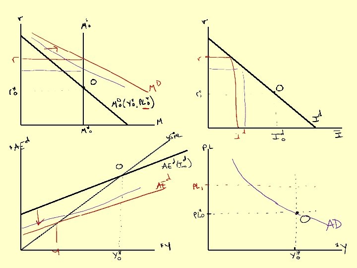
The Aggregate Demand Curve: A Warning u The AD curve is not a market demand curve like in microeconomics. It’s a more complex concept. – It’s an equilibrium locus, really. u Remember: A higher price level causes the demand for money to rise, which causes the interest rate to rise. – Then, the higher interest rate causes aggregate output to fall. – At all points along the AD curve, both the goods market and the money market are in equilibrium.

Additional Reasons for a “Negative” AD Curve u The consumption link: There might be a decrease in consumption brought about by the increase in the interest rate brought about by a higher price level – this would contribute to the overall decrease in aggregate output (Y). u The real wealth effect, or real balance effect: There might be a decrease in consumption brought about by the decrease in real wealth that results from an increase in the price level – this would contribute to the overall decrease in aggregate output (Y). u Note: These are not directly in the model we’ve constructed. . . but you will see them later if you take more macro.

Shifts in Aggregate Demand via Monetary Policy u An increase in Ms at a given price level shifts the aggregate demand curve to the right. u A decrease in Ms at a given price level shifts the aggregate demand curve to the left.

Shifts in Aggregate Demand via Fiscal Policy u An increase in G or a decrease in net T at a given price level shifts the aggregate demand curve to the right. u A decrease in G or an increase in net T at a given price level shifts the aggregate demand curve to the left.

How an increase in the money supply shifts AD to the right.