Acoustic Signal Processing Curt A L Szuberla

Acoustic Signal Processing ▫ Curt A. L. Szuberla ▫ Geophysical Institute, University of Alaska Fairbanks Presented at the Physical Acoustics Summer School La Cienega, NM 28 May 2008

Abstract Between the collection and interpretation of acoustic data lies the art and science of acoustic signal processing. The scientific aspect is rather obvious; it embraces the underlying physics, mathematical and statistical formulations, as well as the computational science and engineering brought to bear. Often overlooked is the art involved. From among the myriad techniques available, we’re required to select the method(s) that will enable us to extract the most meaningful information from the data. Too often, our knowledge of the physics – acoustic source, propagation media and even sensor characteristics – is incomplete, so elements of judgment and experience necessarily come into play. Signal Processing • PASS 2008 2

Abstract (cont’d) For the sake of continuity with the morning’s lecture and in keeping with my own research interests, this lecture will focus on techniques that are useful in the processing of infrasonic data; however, recognize that these methods are not specific in their application, and are applicable to most any area of acoustics. Infrasound signal processing is only used here as a convenient means of illustrating some fundamental concepts. The lecture will follow along the lines of a general pipeline for data processing called PDEC: preprocessing, detection, estimation and classification. It is through this pipeline that all of my research group’s infrasound data flows. Signal Processing • PASS 2008 3

Abstract (cont’d) Acoustic data, in raw form, are not always useful for analysis, so some amount of preprocessing is typically required. Application of filters to the data is the most common form of preprocessing, and several examples will be presented here. Once the data are preprocessed, it is incumbent upon us to detect whether or not a signal of interest is present, and to what degree. This leads to a statistical description of the detection algorithm, or receiver operating characteristic (ROC) curve. Signal Processing • PASS 2008 4

Abstract (cont’d) After a signal of interest is detected, we begin to estimate parameters from the data. These parameters are measures of information carried by the signal and can take on many forms. In particular, this lecture will focus on spectral content and the parameters derived from time difference of arrival (TDOA) information: signal source bearing, elevation, local sound speed and range. The latter parameters are particularly important in the study of array processing. Finally, either in parallel or serial association with parameter estimation, our task is to classify the signal of interest. In many cases this may involve drawing a distinction between source mechanisms or separating a particular source from among clutter or noise. Signal Processing • PASS 2008 5

Abstract (cont’d) Facility in the art and science of acoustic signal processing is tempered by two meta-principles. First, it is necessary to have an intimate knowledge of the characteristics of any technique applied to data. Each technique carries with it a set of assumptions, advantages and limitations. The best way to develop a sense for these properties is to simply play with the techniques, gaining experience by applying them to both actual and contrived data sets. In this manner, one begins to gain an appreciation for what information a particular method can extract from the data. Second, we must have the ability to separate physical results from non-physical ones. Signal Processing • PASS 2008 6

Abstract (cont’d) A colleague of mine from graduate school was fond summing up the whole of signal processing in the phrase, “bumps is bumps and wiggles is wiggles. ” He meant that the techniques of signal processing are broadly applicable to data, data of any kind. Whether you continue with your study of acoustics or branch out into a field as diverse as the financial markets, the ideas presented in this lecture will hopefully serve as a springboard for your own interests in signal processing. Signal Processing • PASS 2008 7

Overview ▫ Bold assertion: Learn all of signal processing in a single, convenient 3 -hour session! ▫ Small-type Disclaimer: Not quite. ▫ Background ▫ A little bit about me ▫ A little bit about you ▫ What we’re about to do Signal Processing • PASS 2008 8

Before We Begin ▫ In [our] experience, the fast computers which are now available are more than adequate for the purposes of spectral analysis. Our present computing facilities are greatly in excess of our ability to make sense of practical data. - Jenkins & Watts, 1968 Signal Processing • PASS 2008 9

th’ Canon ▫ Jenkins & Watts, 1968 ▫ Spectral Analysis and its Applications ▫ Bracewell, 1999 ▫ The Fourier Transform and its Applications ▫ Therrien, 1992 ▫ Discrete Random Signals and Statistical Signal Processing ▫ Press, et al. , 2008 ▫ Numerical Recipes Signal Processing • PASS 2008 10

Preliminaries ▫ ▫ ▫ Notation Discrete Fourier theory Nyquist’s theorem Assumptions Confidence limits Signal Processing • PASS 2008 11

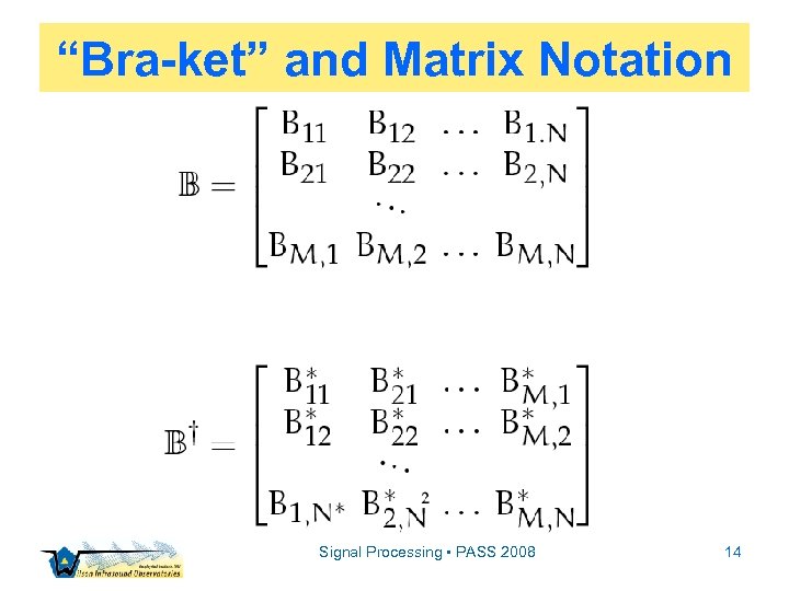
Notation ▫ Data are sampled from continuous quantities in the form of time series ▫ Time series are representable as vectors ▫ The mechanics of matrix notation is therefore handy ▫ We’ll use Dirac’s “bra-ket” notation Signal Processing • PASS 2008 12

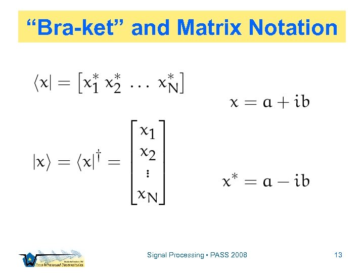
“Bra-ket” and Matrix Notation Signal Processing • PASS 2008 13

“Bra-ket” and Matrix Notation Signal Processing • PASS 2008 14

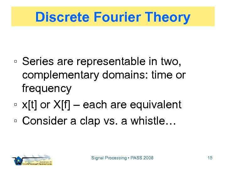
Discrete Fourier Theory ▫ Series are representable in two, complementary domains: time or frequency ▫ x[t] or X[f] – each are equivalent ▫ Consider a clap vs. a whistle… Signal Processing • PASS 2008 15

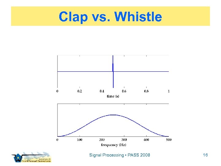
Clap vs. Whistle Signal Processing • PASS 2008 16

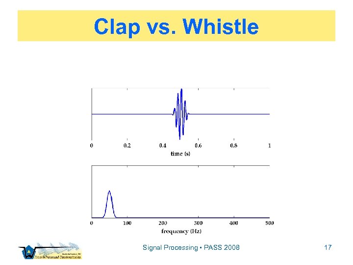
Clap vs. Whistle Signal Processing • PASS 2008 17

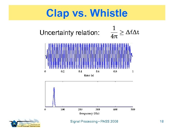
Clap vs. Whistle Uncertainty relation: Signal Processing • PASS 2008 18

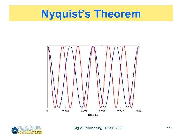
Nyquist’s Theorem Signal Processing • PASS 2008 19

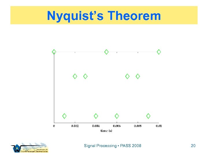
Nyquist’s Theorem Signal Processing • PASS 2008 20

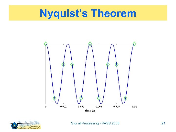
Nyquist’s Theorem Signal Processing • PASS 2008 21

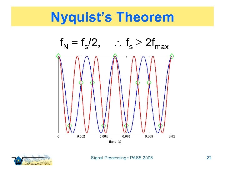
Nyquist’s Theorem f. N = fs/2, fs 2 fmax Signal Processing • PASS 2008 22

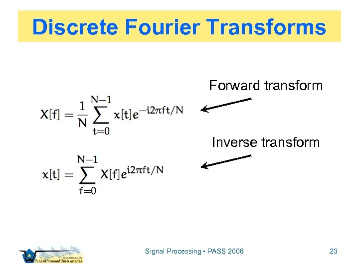
Discrete Fourier Transforms Forward transform Inverse transform Signal Processing • PASS 2008 23

Discrete Fourier Transforms x[t] = [ -1 -0. 4 0. 2 0. 5 0. 8 0. 4 0 -0. 5] Time series DC (mean) Fourier transform Nyquist X[f] = [ 0 -3. 07 -0. 34 i -0. 4 -0. 53+0. 06 i 0 -0. 53 -0. 06 i -0. 4 -3. 07+0. 34 i] Signal Processing • PASS 2008 24

Discrete Fourier Transforms x[t] = [ -1 -0. 4 t = 1/fs 0. 2 0. 5 0. 8 0. 4 0 -0. 5] f f = fs/N X[f] = [ 0 -3. 07 -0. 34 i -0. 4 -0. 53+0. 06 i 0 -0. 53 -0. 06 i -0. 4 -3. 07+0. 34 i] Signal Processing • PASS 2008 25

Power Spectra x[t] X[f]·X[f]* = X[f] 2 x[t] 2 = X[f] 2/N This is a special case of Plancherel's Theorem Signal Processing • PASS 2008 26

Power Spectra This leads us to define the spectrum: S[f] X[f] 2/N S[f] is only an estimate of the true spectrum St[f] However, as T , S[f] St[f] Unfortunately, S[f] 2 Signal Processing • PASS 2008 27

Assumptions ▫ Stationarity ▫ Periodicicity ▫ Both of these assumptions are effectively always violated! ▫ A critical job skill for a physicist: knowing what you can get away with and when! ▫ Ask the question: “Is it physics or artifacts I’m looking at? ” Signal Processing • PASS 2008 28

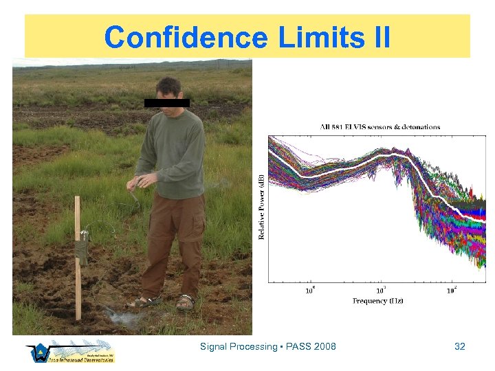
Confidence Limits Statistically, S[f] has only = 2 d. o. f. , (amplitude & phase), which leads to S[f] 2 and it does not decrease as T Happily, we have remedies available… Signal Processing • PASS 2008 29

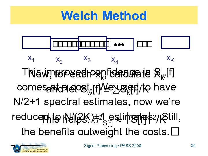
Welch Method x 1 x 2 x 3 x 4 x. K This improved confidence in Xk [f] Now, for each xk, calculate Sw comesandalet Sw[f] Sk[f]/K have at cost. We used to N/2+1 spectral estimates, now we’re reduced to helps: S[f] 2/K This N/(2 K)+1 estimates. Still, the benefits outweight the costs. Signal Processing • PASS 2008 30

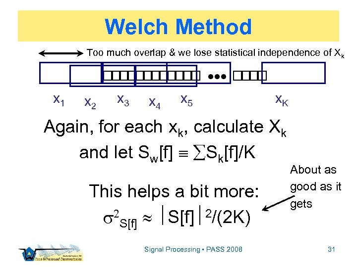
Welch Method Too much overlap & we lose statistical independence of Xk x 1 x 2 x 3 x 4 x 5 x. K Again, for each xk, calculate Xk and let Sw[f] Sk[f]/K This helps a bit more: S[f] 2/(2 K) Signal Processing • PASS 2008 About as good as it gets 31

Confidence Limits II Signal Processing • PASS 2008 32

Infrasound Sensor Demo Signal Processing • PASS 2008 33

Processing Pipeline: PDEC ▫ Preprocessing ▫ Detection ▫ Estimation ▫ Classification Signal Processing • PASS 2008 34

Preprocessing ▫ Filters ▫ Bandpass ▫ Pure State Signal Processing • PASS 2008 35

Bandpass Filtration X[f] DC f 1 f 2 f 3 f. Nyq f 3* f 2* f 1* Signal Processing • PASS 2008 f 36

Bandpass Filtration X[f] DC f 1 f 2 f 3 f. Nyq f 3* f 2* f 1* Signal Processing • PASS 2008 f 37

Bandpass Filtration X[f] DC f 1 f 2 f 3 f. Nyq f 3* f 2* f 1* Signal Processing • PASS 2008 f 38

Bandpass Filtration X[f] DC f 1 f 2 f 3 f. Nyq f 3* f 2* f 1* f To filter, Xbpf[f] xbpf[t] Signal Processing • PASS 2008 39

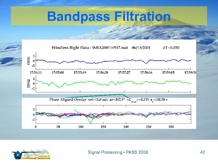
Bandpass Filtration Signal Processing • PASS 2008 40

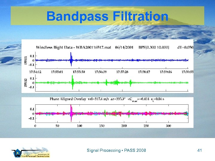
Bandpass Filtration Signal Processing • PASS 2008 41

Pure State Filtration To filter, let Xps[f] = X[f] P[f]c, then Xps[f] xps[t] Signal Processing • PASS 2008 42

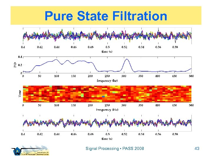
Pure State Filtration Signal Processing • PASS 2008 43

Detection ▫ Detection statistics ▫ Metrics ▫ Thresholds ▫ Receiver Operating Characteristic (ROC) curves Signal Processing • PASS 2008 44

Detection Metrics ▫ Detection: Did something (an event) just happen and are we willing to bet the mortgage on it? ▫ Metric: Some estimable parameter(s) related to event(s) ▫ Typical infrasound metrics: ▫ MCCM (cross correlation) ▫ F-statistic (phase-aligned SNR) Signal Processing • PASS 2008 45

Detection Thresholds ▫ Detection: Did something (an event) just happen and are we willing to bet the mortgage on it? ▫ Threshold: statistical tolerance placed on metric to define event declaration ▫ Receiver Operating Characteristic (ROC) curves are a graphical tool Signal Processing • PASS 2008 46

ROC Curves ▫ Receiver Operating Characteristic (ROC) curves graphically depict detection schemata efficiencies ▫ We’ll consider 1 D ROC w/ a parameter p, estimable from data ▫ Play with www. anaesthetist. com/mnm/stats/roc Signal Processing • PASS 2008 47

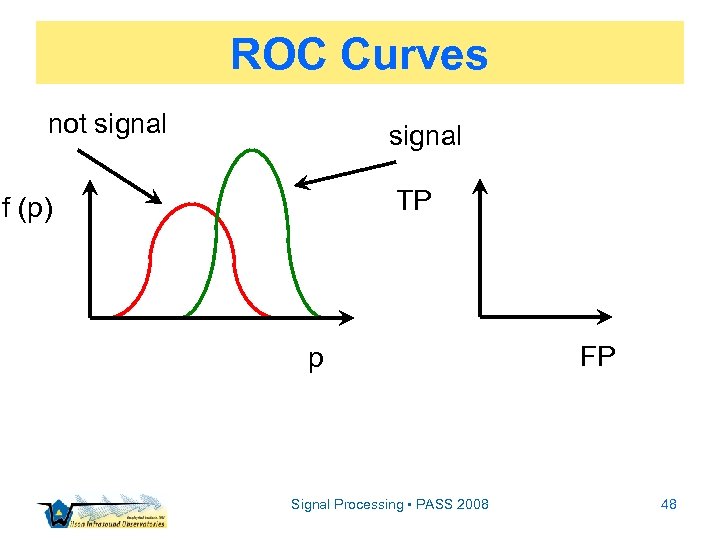
ROC Curves not signal TP f (p) p Signal Processing • PASS 2008 FP 48

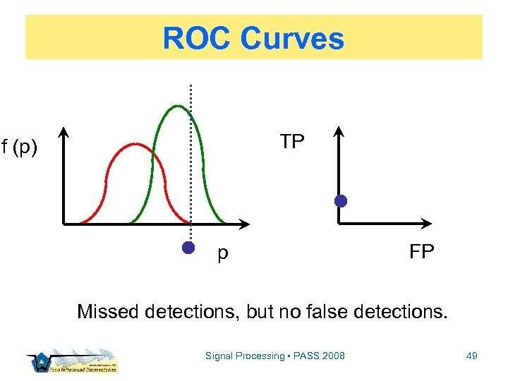
ROC Curves TP f (p) p FP Missed detections, but no false detections. Signal Processing • PASS 2008 49

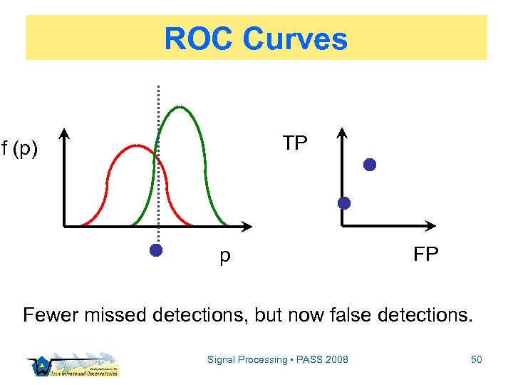
ROC Curves TP f (p) p FP Fewer missed detections, but now false detections. Signal Processing • PASS 2008 50

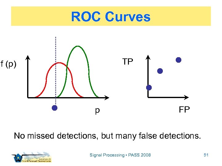
ROC Curves TP f (p) p FP No missed detections, but many false detections. Signal Processing • PASS 2008 51

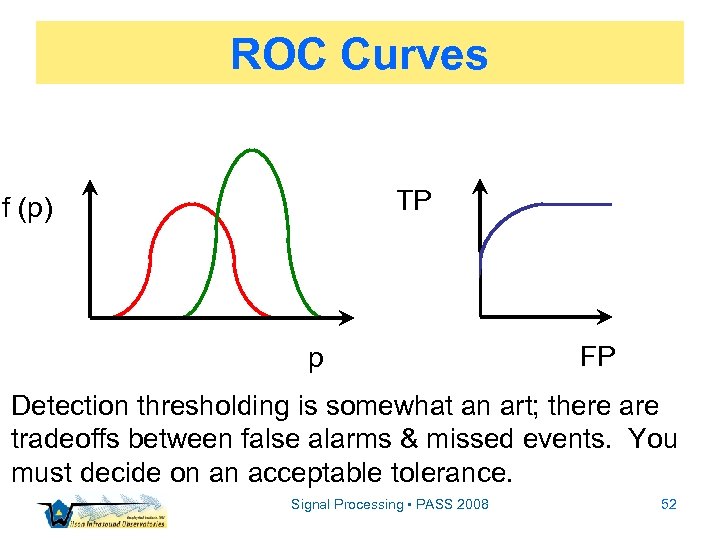
ROC Curves TP f (p) p FP Detection thresholding is somewhat an art; there are tradeoffs between false alarms & missed events. You must decide on an acceptable tolerance. Signal Processing • PASS 2008 52

Estimation ▫ Spectrum Estimation: S ▫ TDOA information: ▫ Correlation: c ▫ Coherence: C ▫ Array processing ▫ Far-field: , vt ▫ Near-field: , vt, r Signal Processing • PASS 2008 53

TDOA Information ▫ Time difference of arrival ▫ Two or more physically distinct sensors and a finite sound speed give rise to TDOA ▫ One approach to array processing ▫ Computationally efficient and effective Signal Processing • PASS 2008 54

Cross Correlation ▫ Perhaps the most useful tool for TDOA information estimation ▫ Estimated as cxy[ ] = x[t+ ] y[t]* ▫ Convolution in the time domain is analogous to multiplication in the frequency domain (attack via FFT) ▫ Can be normalized / generalized Signal Processing • PASS 2008 55

Coherence ▫ Coherence is a frequency-domain analogue of correlation ▫ Like P[f] ▫ It is biased toward unity for small ▫ C[f] & P[f] [0, 1] ▫ Unlike P[f] ▫ Limited to 2 -channel data ▫ Not fooled by 1 -channel loud signals ▫ Not trace-invariant (geometric dependence) Signal Processing • PASS 2008 56

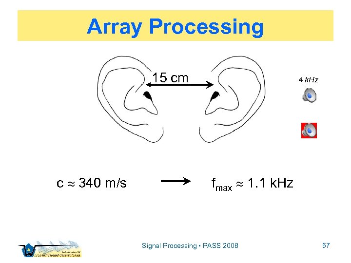
Array Processing 15 cm c 340 m/s 4 k. Hz fmax 1. 1 k. Hz Signal Processing • PASS 2008 57

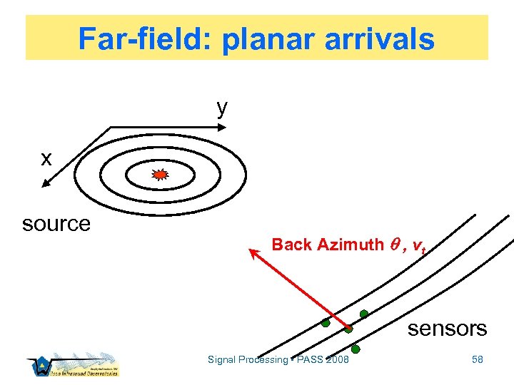
Far-field: planar arrivals y x source Back Azimuth , vt sensors Signal Processing • PASS 2008 58

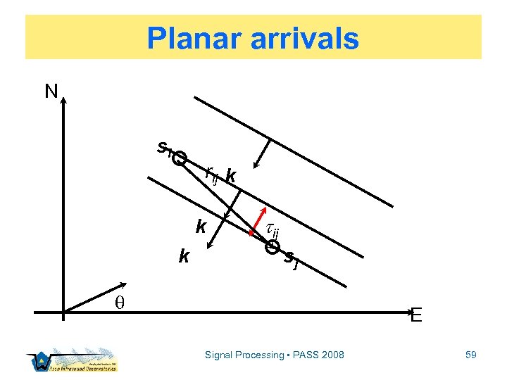
Planar arrivals N si rij k k k ij sj E Signal Processing • PASS 2008 59

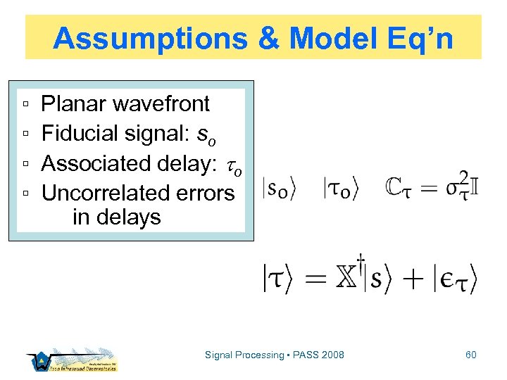
Assumptions & Model Eq’n ▫ ▫ Planar wavefront Fiducial signal: so Associated delay: o Uncorrelated errors in delays Signal Processing • PASS 2008 60

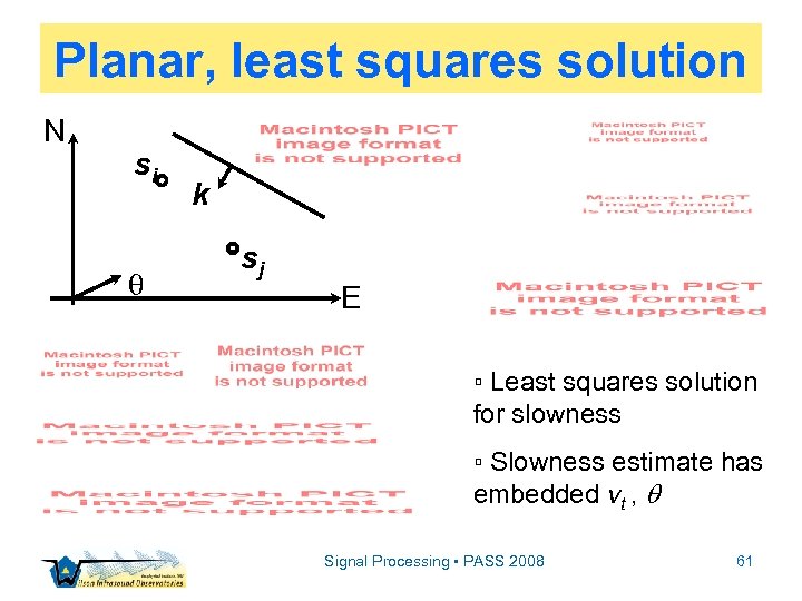
Planar, least squares solution N si k sj E ▫ Least squares solution for slowness ▫ Slowness estimate has embedded vt , Signal Processing • PASS 2008 61

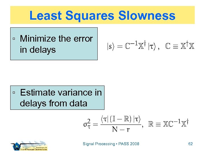
Least Squares Slowness ▫ Minimize the error in delays ▫ Estimate variance in delays from data Signal Processing • PASS 2008 62

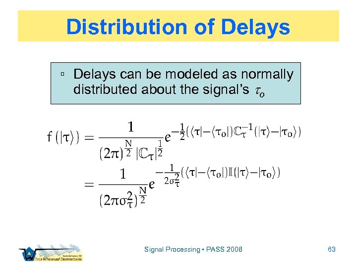
Distribution of Delays ▫ Delays can be modeled as normally distributed about the signal’s o Signal Processing • PASS 2008 63

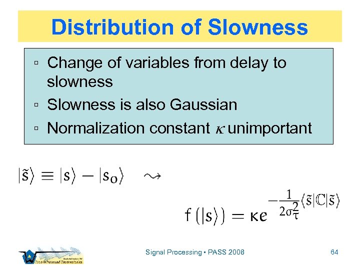
Distribution of Slowness ▫ Change of variables from delay to slowness ▫ Slowness is also Gaussian ▫ Normalization constant k unimportant Signal Processing • PASS 2008 64

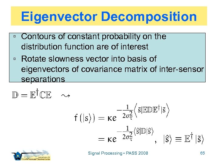
Eigenvector Decomposition ▫ Contours of constant probability on the distribution function are of interest ▫ Rotate slowness vector into basis of eigenvectors of covariance matrix of inter-sensor separations Signal Processing • PASS 2008 65

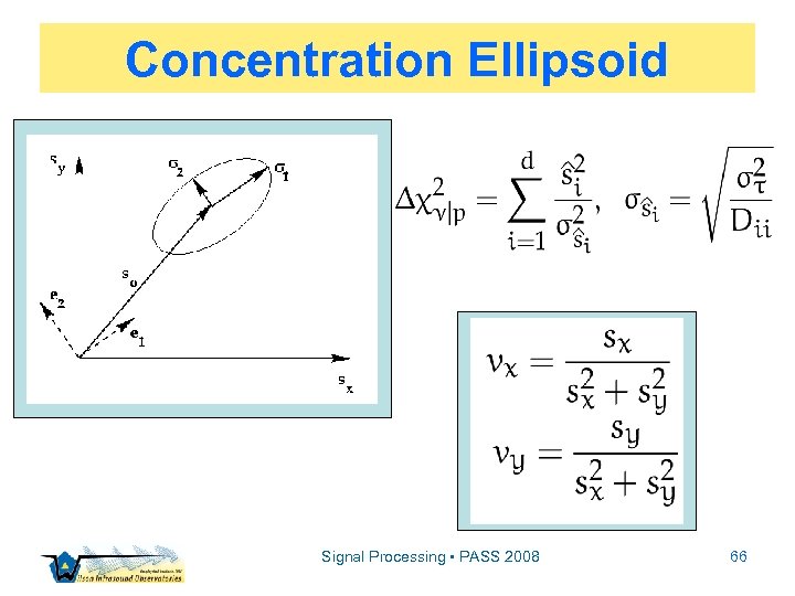
Concentration Ellipsoid Signal Processing • PASS 2008 66

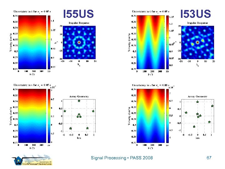
I 55 US Signal Processing • PASS 2008 I 53 US 67

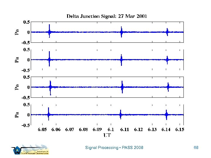
Signal Processing • PASS 2008 68

Signal Processing • PASS 2008 69

Signal Processing • PASS 2008 70

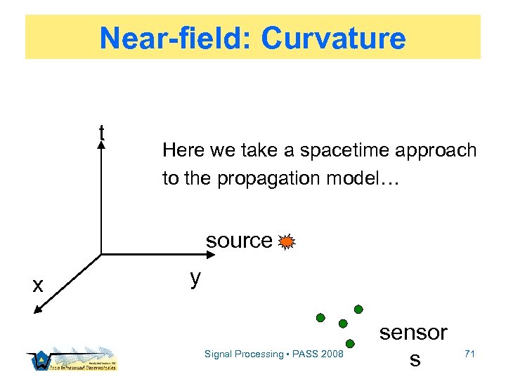
Near-field: Curvature t Here we take a spacetime approach to the propagation model… source x y Signal Processing • PASS 2008 sensor s 71

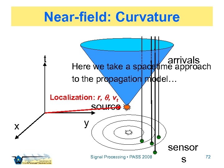
Near-field: Curvature t arrivals Here we take a spacetime approach to the propagation model… Localization: r, , vt source x y Signal Processing • PASS 2008 sensor s 72

Automated Localization 2007 Midnight Sun Run 10 -km Race w/ 75 -mm Cannon Start Gun Finish Guns Signal Processing • PASS 2008 73

2007 MSR: Start Gun Signal Processing • PASS 2008 74

2007 MSR: Finish Guns Signal Processing • PASS 2008 75

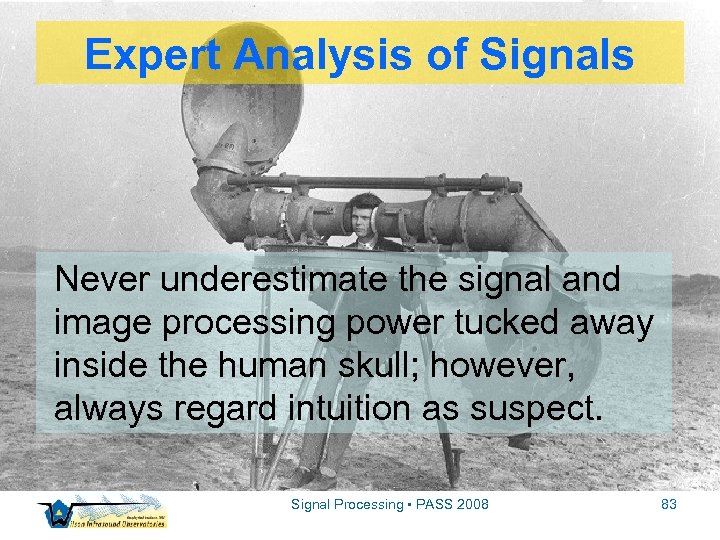
Classification ▫ Frequency-time localization ▫ Expert analysis ▫ Automated techniques Signal Processing • PASS 2008 76

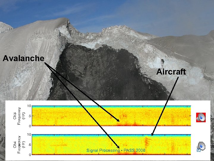
Spectrograms Frequency-time localization is limited by the uncertainty relations. However, if we’re not too demanding we can get an estimate of spectral content as a function of time. Let’s look at a serendipitous example of spectrographic analysis. Signal Processing • PASS 2008 77

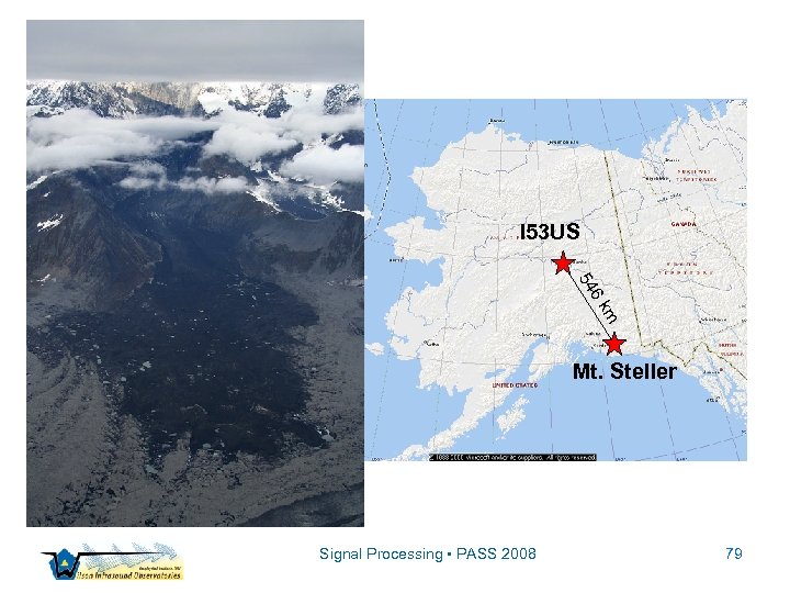
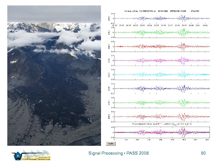
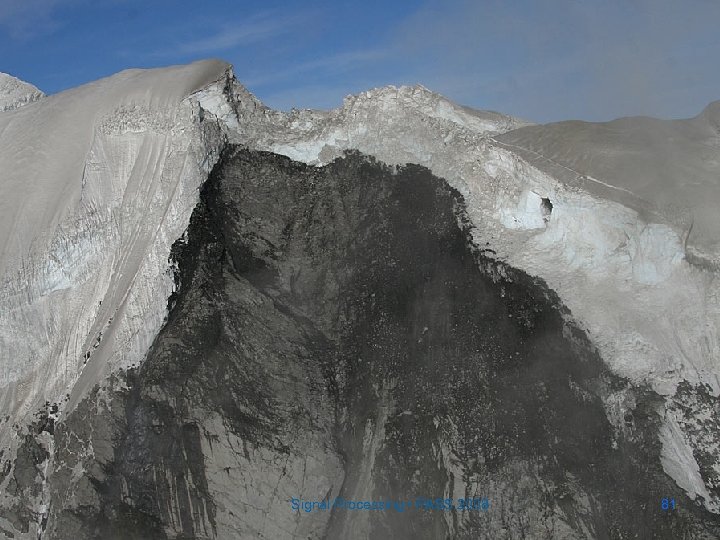
Mt. Steller Avalanche ▫ 14 September 2005: rock & ice avalanche occurred on Mt. Steller ▫ Covered valley floor with debris for ~9 km ▫ Volume displaced ~15 106 m 3 ▫ Event detected by at I 53 US ▫ I 53 US ~550 km away from the mountain Signal Processing • PASS 2008 78

I 53 US 54 m 6 k Mt. Steller Signal Processing • PASS 2008 79

Signal Processing • PASS 2008 80

Signal Processing • PASS 2008 81

Avalanche Aircraft Signal Processing • PASS 2008 82

Expert Analysis of Signals Never underestimate the signal and image processing power tucked away inside the human skull; however, always regard intuition as suspect. Signal Processing • PASS 2008 83

23 Sep 06 House Fire Signal Processing • PASS 2008 84

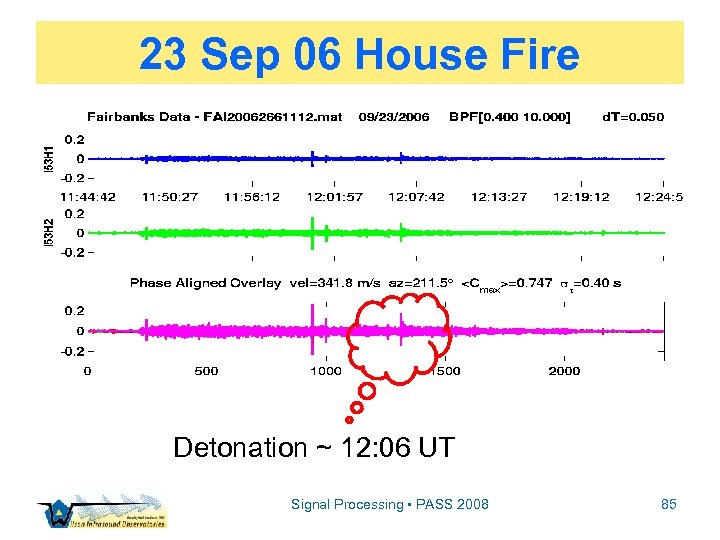
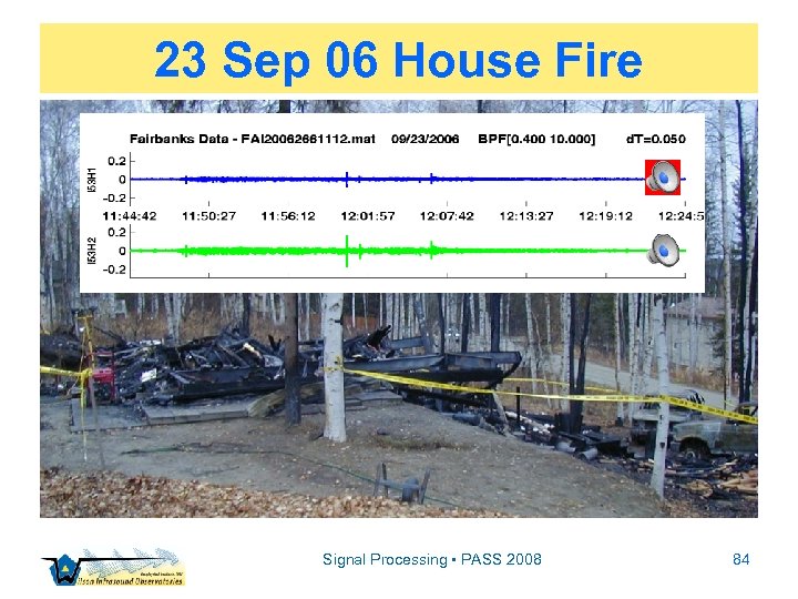
23 Sep 06 House Fire Detonation ~ 12: 06 UT Signal Processing • PASS 2008 85

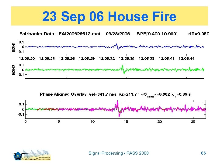
23 Sep 06 House Fire Signal Processing • PASS 2008 86

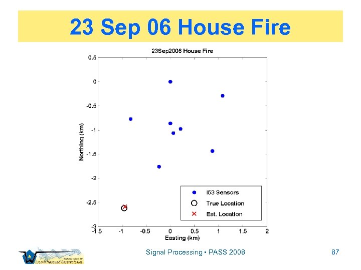
23 Sep 06 House Fire Signal Processing • PASS 2008 87

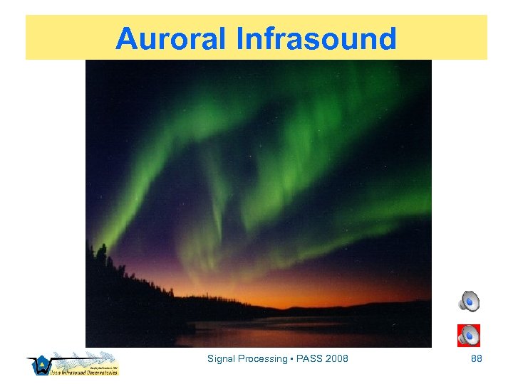
Auroral Infrasound Signal Processing • PASS 2008 88

Automated Classification ▫ Neural networks ▫ One of my graduate students has cracked the HTV vs. MAW problem ▫ The example I won’t commit to slides ▫ An example of the K. I. S. S. principle Signal Processing • PASS 2008 89

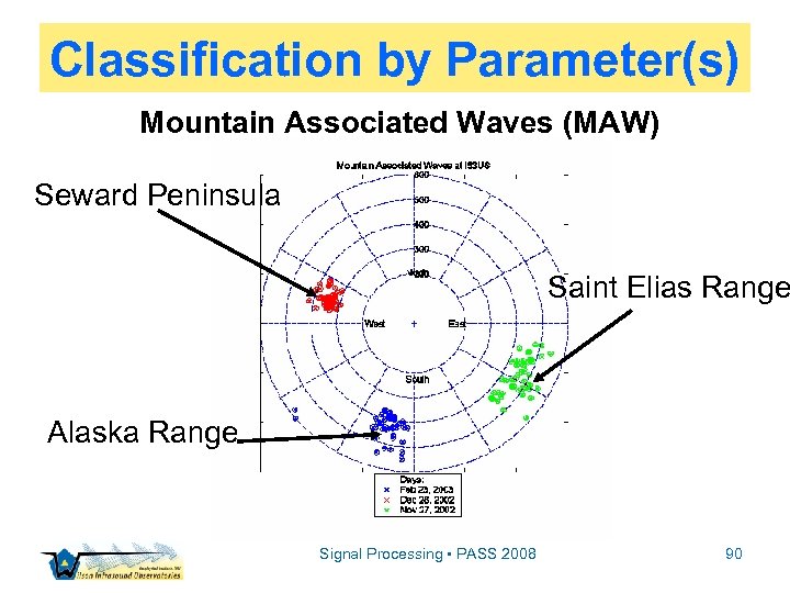
Classification by Parameter(s) Mountain Associated Waves (MAW) Seward Peninsula Saint Elias Range Alaska Range Signal Processing • PASS 2008 90

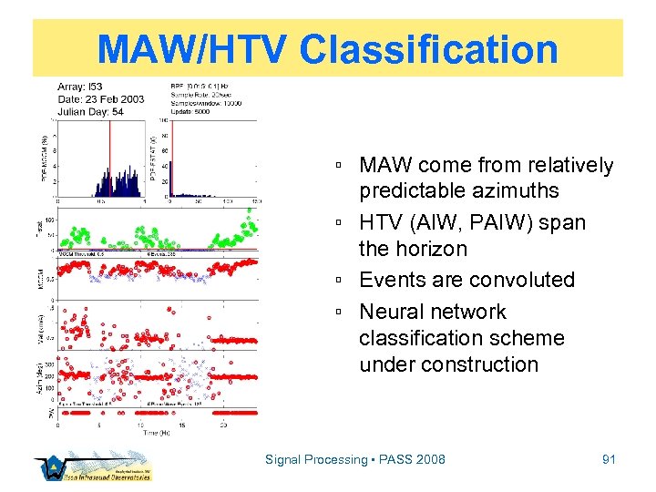
MAW/HTV Classification ▫ MAW come from relatively predictable azimuths ▫ HTV (AIW, PAIW) span the horizon ▫ Events are convoluted ▫ Neural network classification scheme under construction Signal Processing • PASS 2008 91

Unstructured Learning ▫ The single best way to develop a sense for signal processing is to play with its techniques! ▫ Applications are endless: ▫ Actual data ▫ Synthetic data ▫ Combinations of both Signal Processing • PASS 2008 92

Playing with Signal Processing C C++ Signal Processing • PASS 2008 93

True North Mine r ~ 30 km I 53 US ~ 30 Signal Processing • PASS 2008 94

True North Mine Blast Acoustic trace velocity & consistent High azimuth correlation & planar arrival Blast-wave param’s filtered Bandpass T ~ 3 s & tr ~ 0. 2 s above microbarom band Signal Processing • PASS 2008 95

True North Mine & FWA 3 arrays: True North Mine • 8 -element (2 -km aperture) • 6 -element (0. 2 -km aperture) • 14 -element (12 -km aperture) I 53 US FWA d ~ 12 km Signal Processing • PASS 2008 96

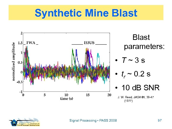
Synthetic Mine Blast parameters: • T~3 s • tr ~ 0. 2 s • 10 d. B SNR J. W. Reed, JASA 61, 39 -47 (1977) Signal Processing • PASS 2008 97

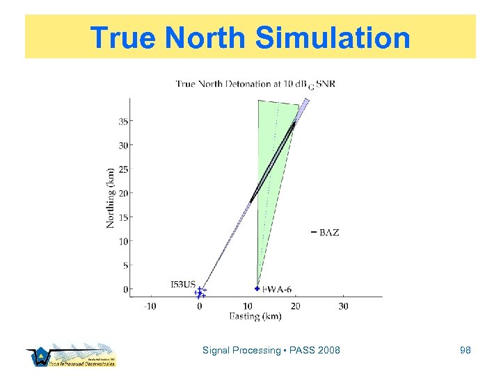
True North Simulation Signal Processing • PASS 2008 98

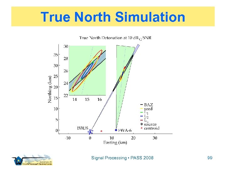
True North Simulation Signal Processing • PASS 2008 99

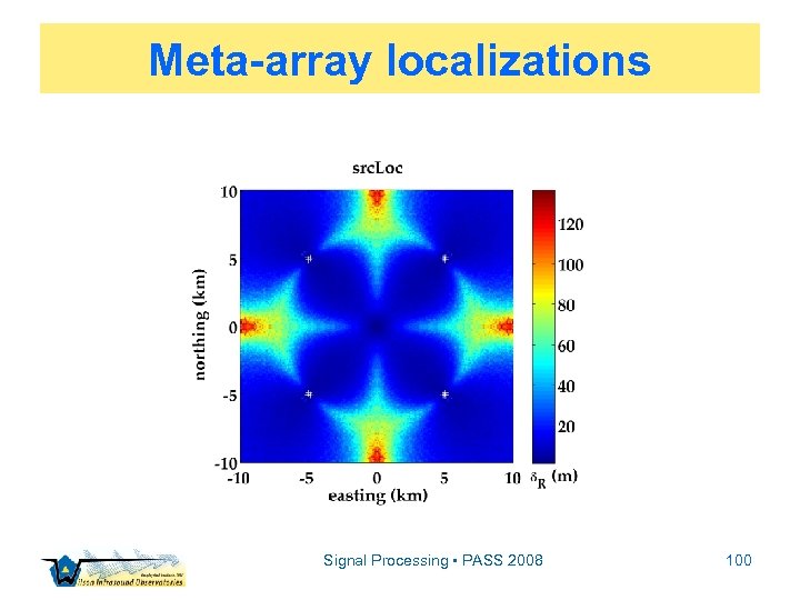
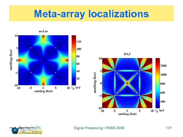
Meta-array localizations Signal Processing • PASS 2008 100

Meta-array localizations Signal Processing • PASS 2008 101

“That’s All Folks…” ▫ The complete Power. Point presentation of this talk and selected references are available: www. gi. alaska. edu/~cas/physics/PASS 08 ▫ Contact me: cas@gi. alaska. edu ▫ Hopefully this quick tour will whet your appetite for signal processing Signal Processing • PASS 2008 102