ACAI 05 SEKT 05 ADVANCED COURSE ON KNOWLEDGE DISCOVERY

ACAI’ 05/SEKT’ 05 ADVANCED COURSE ON KNOWLEDGE DISCOVERY Distributed Data Mining Dr. Giuseppe Di Fatta University of Konstanz (Germany) and ICAR-CNR, Palermo (Italy) 5 July, 2005 1 Email: fatta@inf. uni-konstanz. de, difatta@pa. icar. cnr. it

Tutorial Outline Ø Part 1: Overview of High-Performance Computing Ø Technology trends Ø Parallel and Distributed Computing architectures Ø Programming paradigms Ø Part 2: Distributed Data Mining Ø Classification Ø Clustering Ø Association Rules Ø Graph Mining Ø Conclusions 2

Tutorial Outline Ø Part 1: Overview of High-Performance Computing Ø Technology trends § § Processing § Memory § Communication § 3 Moore’s law Supercomputers

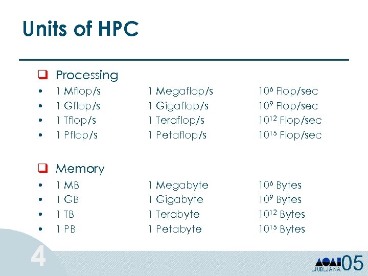Units of HPC q Processing • • 1 Mflop/s 1 Gflop/s 1 Tflop/s 1 Pflop/s 1 Megaflop/s 1 Gigaflop/s 1 Teraflop/s 1 Petaflop/s 106 Flop/sec 109 Flop/sec 1012 Flop/sec 1015 Flop/sec 1 Megabyte 1 Gigabyte 1 Terabyte 1 Petabyte 106 Bytes 109 Bytes 1012 Bytes 1015 Bytes q Memory • • 4 1 MB 1 GB 1 TB 1 PB

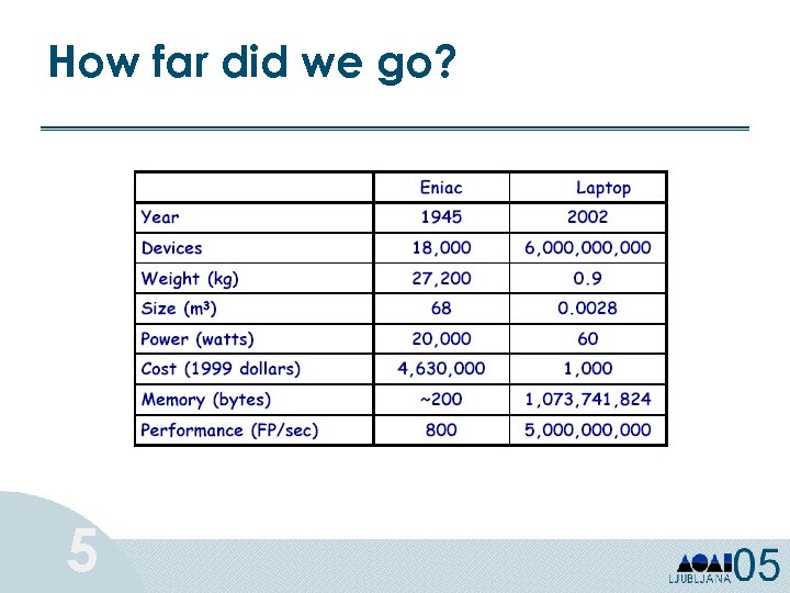How far did we go? 5

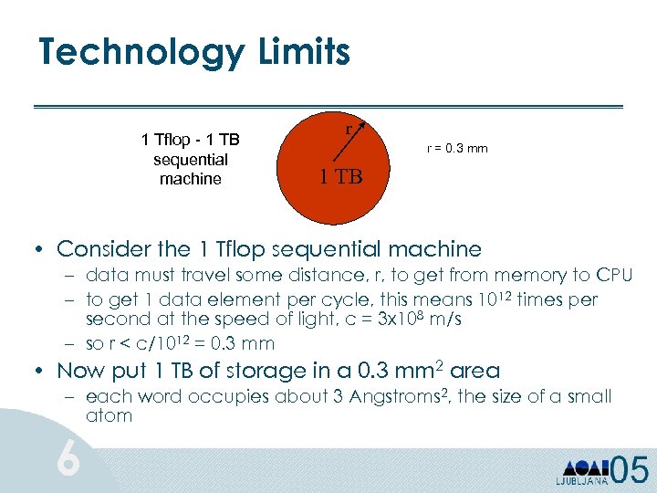Technology Limits 1 Tflop - 1 TB sequential machine r r = 0. 3 mm 1 TB • Consider the 1 Tflop sequential machine – data must travel some distance, r, to get from memory to CPU – to get 1 data element per cycle, this means 1012 times per second at the speed of light, c = 3 x 108 m/s – so r < c/1012 = 0. 3 mm • Now put 1 TB of storage in a 0. 3 mm 2 area – each word occupies about 3 Angstroms 2, the size of a small atom 6

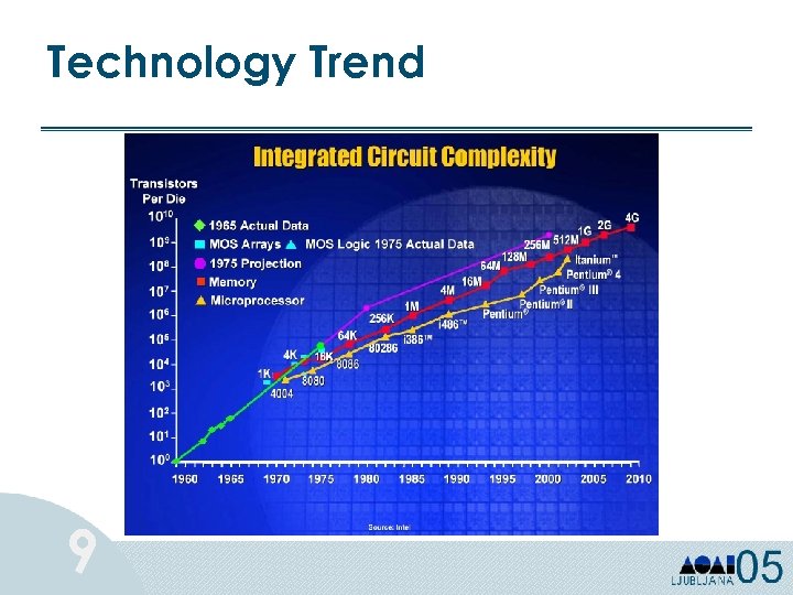
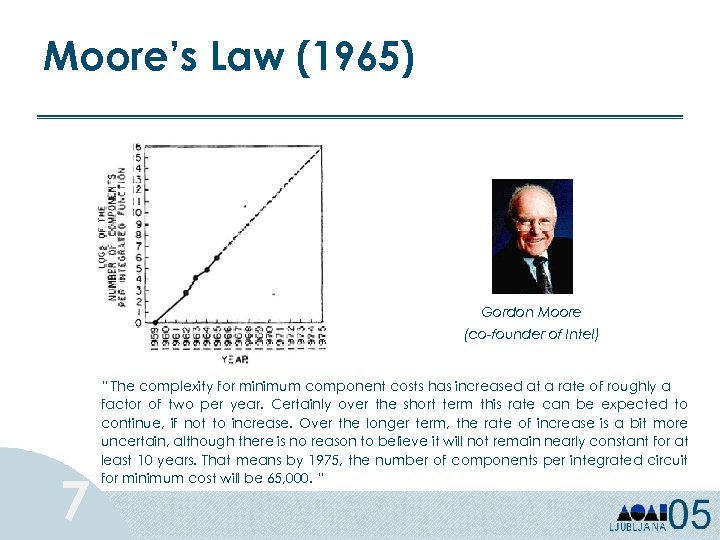Moore’s Law (1965) Gordon Moore (co-founder of Intel) 7 “ The complexity for minimum component costs has increased at a rate of roughly a factor of two per year. Certainly over the short term this rate can be expected to continue, if not to increase. Over the longer term, the rate of increase is a bit more uncertain, although there is no reason to believe it will not remain nearly constant for at least 10 years. That means by 1975, the number of components per integrated circuit for minimum cost will be 65, 000. “

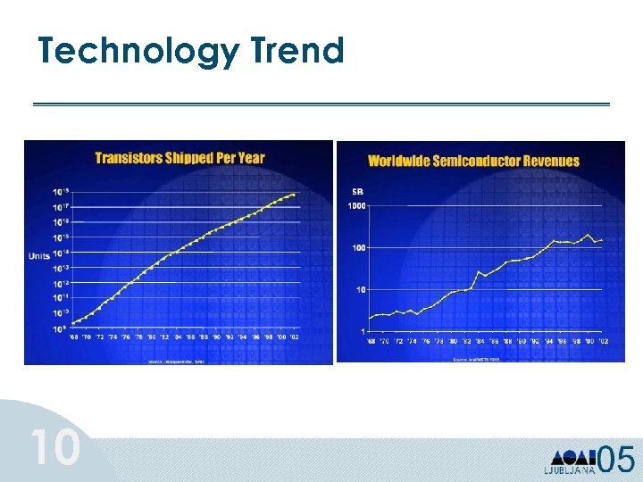
Moore’s Law (1975) In 1975, Moore refined his law: circuit complexity doubles every 18 months. Ø So far it holds for CPUs and DRAMs! Ø Extrapolation for computing power at a given cost and semiconductor revenues. 8

Technology Trend 9

Technology Trend 10

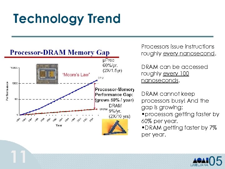Technology Trend Processors issue instructions roughly every nanosecond. DRAM can be accessed roughly every 100 nanoseconds. DRAM cannot keep processors busy! And the gap is growing: • processors getting faster by 60% per year. • DRAM getting faster by 7% per year. 11

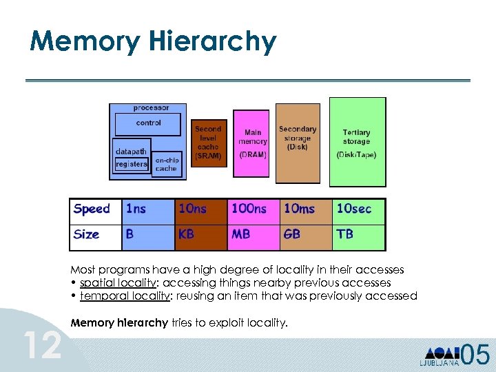Memory Hierarchy Most programs have a high degree of locality in their accesses • spatial locality: accessing things nearby previous accesses • temporal locality: reusing an item that was previously accessed 12 Memory hierarchy tries to exploit locality.

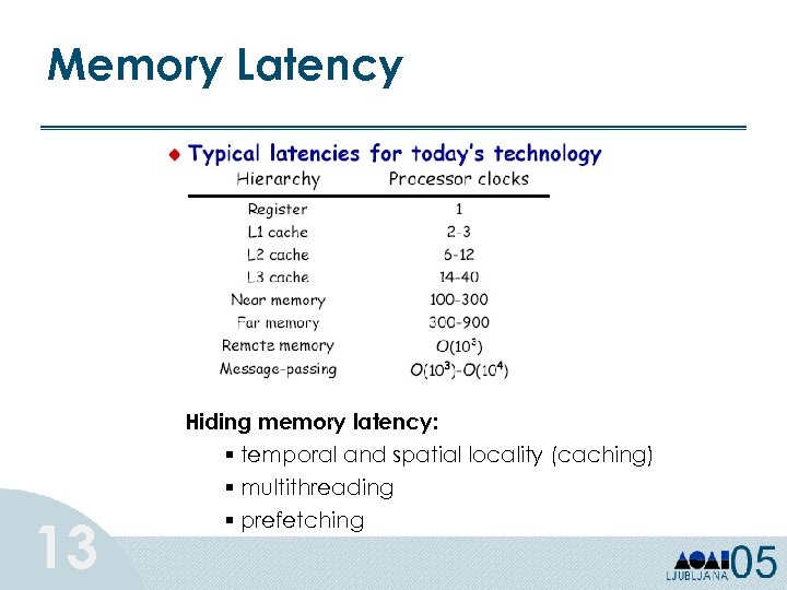Memory Latency 13 Hiding memory latency: § temporal and spatial locality (caching) § multithreading § prefetching

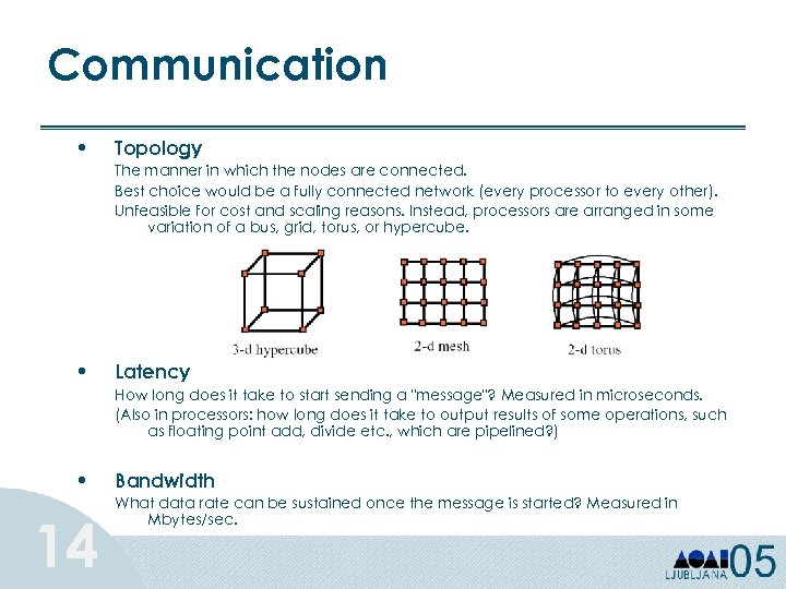Communication • Topology The manner in which the nodes are connected. Best choice would be a fully connected network (every processor to every other). Unfeasible for cost and scaling reasons. Instead, processors are arranged in some variation of a bus, grid, torus, or hypercube. • Latency How long does it take to start sending a "message"? Measured in microseconds. (Also in processors: how long does it take to output results of some operations, such as floating point add, divide etc. , which are pipelined? ) • 14 Bandwidth What data rate can be sustained once the message is started? Measured in Mbytes/sec.

Networking Trend System interconnection network: • bus, crossbar, array, mesh, tree • static, dynamic • LAN/WAN 15

LAN/WAN § 1 st network connection in 1969: 50 Kpbs at about 10: 30 PM on October 29'th, 1969, the first ARPANET connection was established between UCLA and SRI over a 50 kbps line provided by the AT&T telephone company. “At the UCLA end, they typed in the 'l' and asked SRI if they received it; 'got the l' came the voice reply. UCLA typed in the 'o', asked if they got it, and received 'got the o'. UCLA then typed in the 'g' and the darned system CRASHED! Quite a beginning. On the second attempt, it worked fine!” (Leonard Kleinrock) § 10 Base 5 Ethernet in 1976 by Bob Metcalfe and David Boggs § end of ‘ 90 s: 100 Mbps (fast Ethernet) and 1 Gbps Bandwidth is not all the story! Do not forget to consider delay and latency. 16

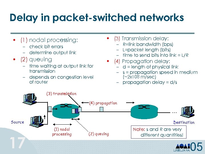Delay in packet-switched networks • (3) Transmission delay: • (1) nodal processing: – R=link bandwidth (bps) – L=packet length (bits) – time to send bits into link = L/R – check bit errors – determine output link • (2) queuing – time waiting at output link for transmission – depends on congestion level of router • (4) Propagation delay: – d = length of physical link – s = propagation speed in medium (~2 x 108 m/sec) – propagation delay = d/s (3) transmission (4) propagation … Source 17 Destination (1) nodal processing (2) queuing Note: s and R are very different quantities!

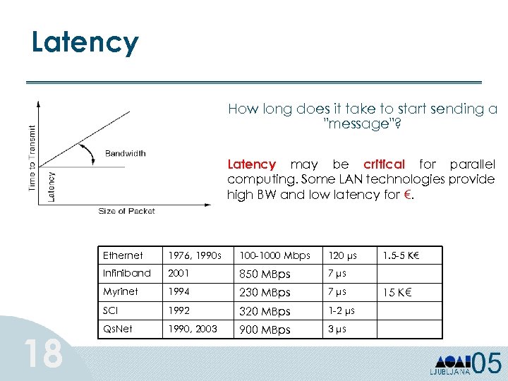Latency How long does it take to start sending a "message"? Latency may be critical for parallel computing. Some LAN technologies provide high BW and low latency for €. Ethernet 100 -1000 Mbps 120 μs Infiniband 2001 850 MBps 7 μs Myrinet 1994 230 MBps 7 μs SCI 18 1976, 1990 s 1992 320 MBps 1 -2 μs Qs. Net 1990, 2003 900 MBps 3 μs 1. 5 -5 K€ 15 K€

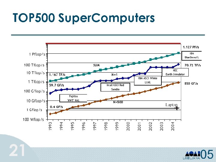
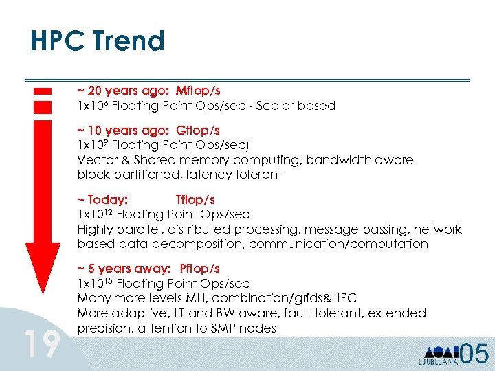HPC Trend ~ 20 years ago: Mflop/s 1 x 106 Floating Point Ops/sec - Scalar based ~ 10 years ago: Gflop/s 1 x 109 Floating Point Ops/sec) Vector & Shared memory computing, bandwidth aware block partitioned, latency tolerant ~ Today: Tflop/s 1 x 1012 Floating Point Ops/sec Highly parallel, distributed processing, message passing, network based data decomposition, communication/computation 19 ~ 5 years away: Pflop/s 1 x 1015 Floating Point Ops/sec Many more levels MH, combination/grids&HPC More adaptive, LT and BW aware, fault tolerant, extended precision, attention to SMP nodes

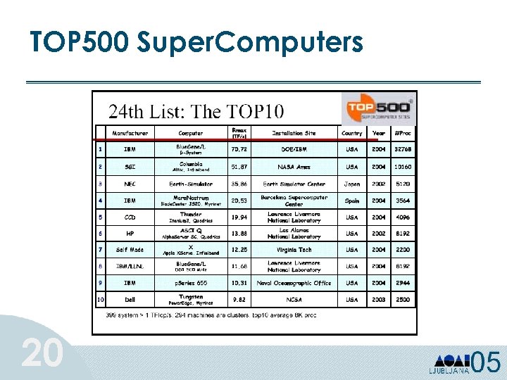TOP 500 Super. Computers 20

TOP 500 Super. Computers 21

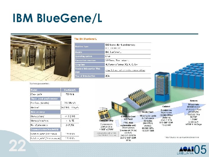IBM Blue. Gene/L 22

Tutorial Outline Ø Part 1: Overview of High-Performance Computing Ø Technology trends Ø Parallel and Distributed Computing architectures Ø Programming paradigms 23

Parallel and Distributed Systems 24

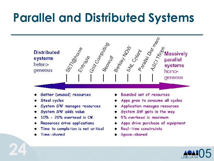
Different Architectures • Parallel computing single systems with many processors working on same problem • Distributed computing many systems loosely coupled by a scheduler to work on related problems • Grid Computing (Meta. Computing) many systems tightly coupled by software, perhaps geographically distributed, to work together on single problems or on related problems Massively Parallel Processors (MPPs) continue to account of more than half of all installed high-performance computers worldwide (Top 500 list). Microprocessor based supercomputers have brought a major change in accessibility and affordability. Nowadays, cluster systems are the most growing part. 25

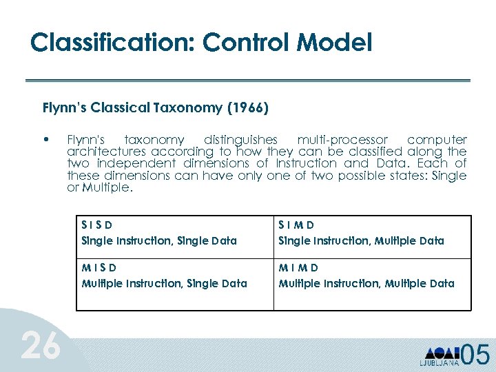Classification: Control Model Flynn’s Classical Taxonomy (1966) • Flynn's taxonomy distinguishes multi-processor computer architectures according to how they can be classified along the two independent dimensions of Instruction and Data. Each of these dimensions can have only one of two possible states: Single or Multiple. SISD Single Instruction, Single Data MISD Multiple Instruction, Single Data 26 SIMD Single Instruction, Multiple Data MIMD Multiple Instruction, Multiple Data

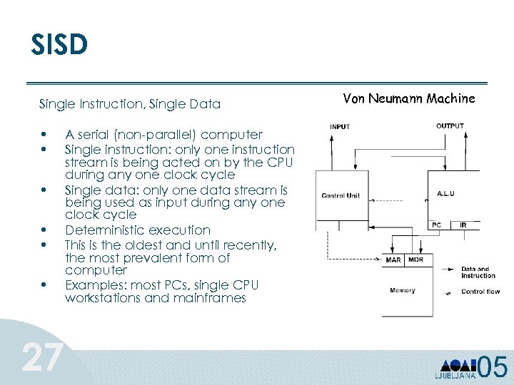SISD Single Instruction, Single Data • • • 27 A serial (non-parallel) computer Single instruction: only one instruction stream is being acted on by the CPU during any one clock cycle Single data: only one data stream is being used as input during any one clock cycle Deterministic execution This is the oldest and until recently, the most prevalent form of computer Examples: most PCs, single CPU workstations and mainframes Von Neumann Machine

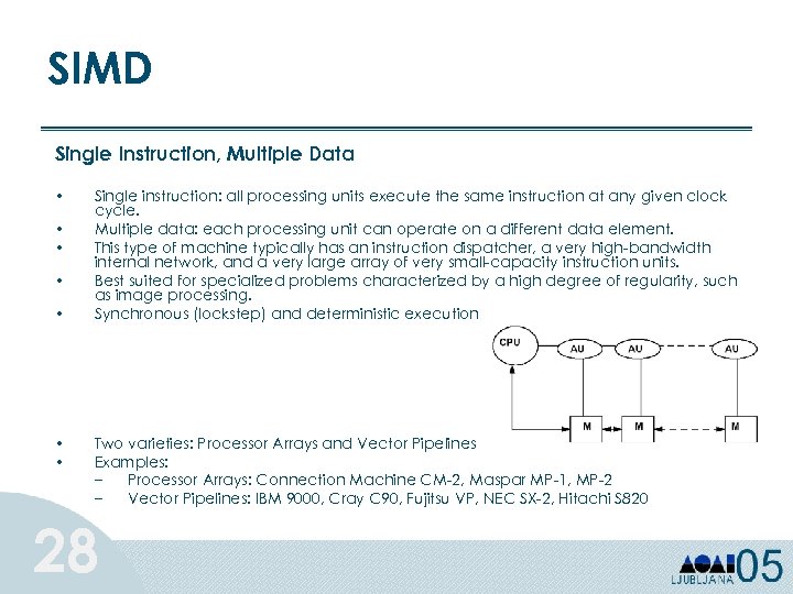SIMD Single Instruction, Multiple Data • • Single instruction: all processing units execute the same instruction at any given clock cycle. Multiple data: each processing unit can operate on a different data element. This type of machine typically has an instruction dispatcher, a very high-bandwidth internal network, and a very large array of very small-capacity instruction units. Best suited for specialized problems characterized by a high degree of regularity, such as image processing. Synchronous (lockstep) and deterministic execution Two varieties: Processor Arrays and Vector Pipelines Examples: – Processor Arrays: Connection Machine CM-2, Maspar MP-1, MP-2 – Vector Pipelines: IBM 9000, Cray C 90, Fujitsu VP, NEC SX-2, Hitachi S 820 28

MISD Multiple Instruction, Single Data • • 29 Few actual examples of this class of parallel computer have ever existed. Some conceivable examples might be: – – multiple frequency filters operating on a single signal stream multiple cryptography algorithms attempting to crack a single coded message.

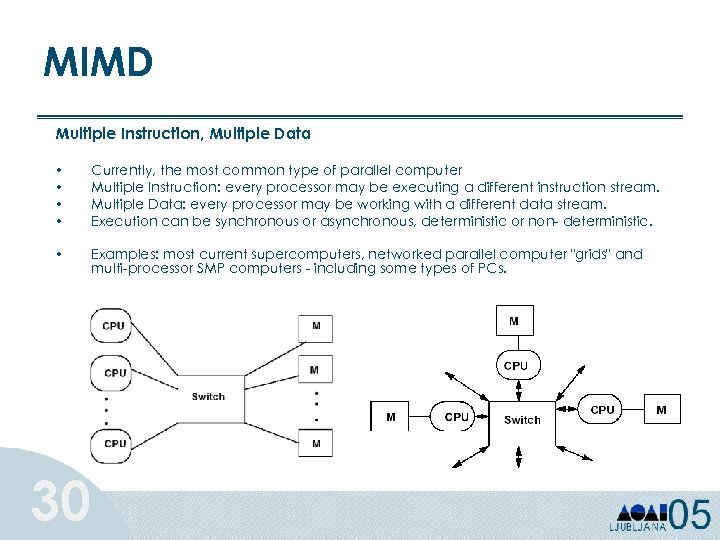MIMD Multiple Instruction, Multiple Data • • Currently, the most common type of parallel computer Multiple Instruction: every processor may be executing a different instruction stream. Multiple Data: every processor may be working with a different data stream. Execution can be synchronous or asynchronous, deterministic or non- deterministic. • Examples: most current supercomputers, networked parallel computer "grids" and multi-processor SMP computers - including some types of PCs. 30

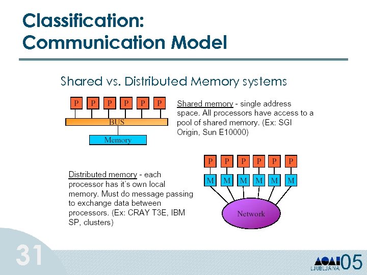Classification: Communication Model Shared vs. Distributed Memory systems 31

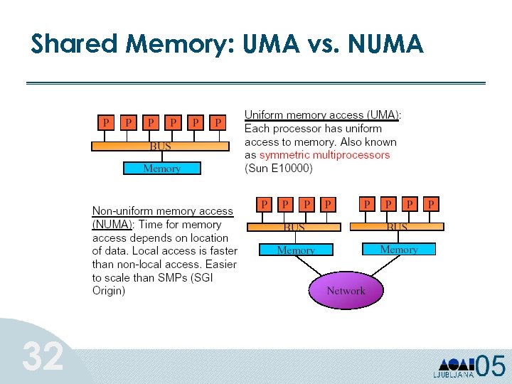Shared Memory: UMA vs. NUMA 32

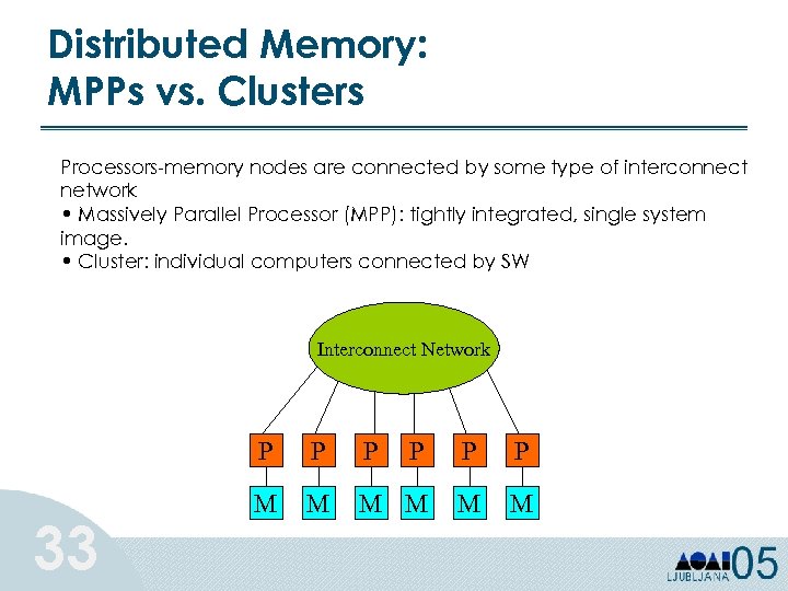Distributed Memory: MPPs vs. Clusters Processors-memory nodes are connected by some type of interconnect network • Massively Parallel Processor (MPP): tightly integrated, single system image. • Cluster: individual computers connected by SW Interconnect Network P 33 P P P M M M

Distributed Shared-Memory Virtual shared memory (shared address space) • on hardware level • on software level Global address space spanning all of the memory in the system. E. g. , HPF, Tread. Marks, sw for No. W (Java. Party, Manta, Jackal) 34

Parallel vs. Distributed Computing q Parallel computing usually considers dedicated homogeneous HPC systems to solve parallel problems. q Distributed computing extends the parallel approach to heterogeneous general-purpose systems. q Both look at the parallel formulation of a problem. q But usually reliability, security, heterogeneity are not considered in parallel computing. But they are considered in Grid computing. “A distributed system is one in which the failure of a computer you didn't even know existed can render your own computer unusable. ” (Leslie Lamport) 35

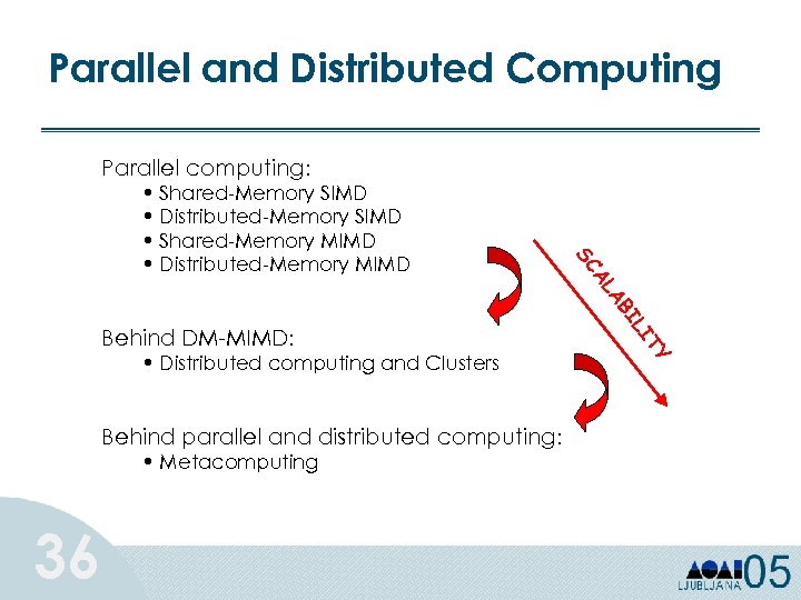Parallel and Distributed Computing Parallel computing: • Metacomputing 36 Y IT Behind parallel and distributed computing: IL • Distributed computing and Clusters AB AL Behind DM-MIMD: SC • Shared-Memory SIMD • Distributed-Memory SIMD • Shared-Memory MIMD • Distributed-Memory MIMD

Tutorial Outline Ø Part 1: Overview of High-Performance Computing Ø Technology trends Ø Parallel and Distributed Computing architectures Ø Programming paradigms § § Problem decomposition § 37 Programming models Parallel programming issues

Programming Paradigms Parallel Programming Models • Control • Naming • Set of operations • Cost 38 – – – – how is parallelism created what orderings exist between operations how do different threads of control synchronize what data is private vs. shared how logically shared data is accessed or communicated what are the basic operations what operations are considered to be atomic how do we account for the cost of each of the above

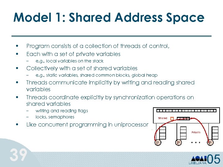Model 1: Shared Address Space • • Program consists of a collection of threads of control, Each with a set of private variables – • Collectively with a set of shared variables – • • e. g. , static variables, shared common blocks, global heap Threads communicate implicitly by writing and reading shared variables Threads coordinate explicitly by synchronization operations on shared variables – – • e. g. , local variables on the stack writing and reading flags locks, semaphores Like concurrent programming in uniprocessor 39

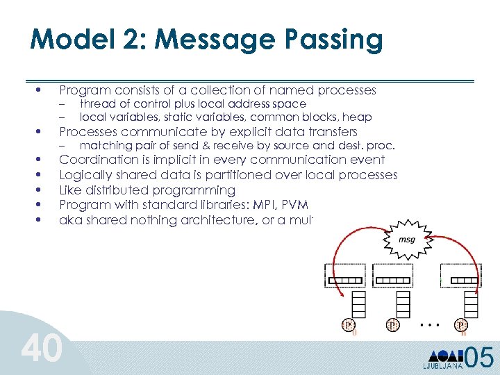Model 2: Message Passing • Program consists of a collection of named processes • Processes communicate by explicit data transfers • • • – – – thread of control plus local address space local variables, static variables, common blocks, heap matching pair of send & receive by source and dest. proc. Coordination is implicit in every communication event Logically shared data is partitioned over local processes Like distributed programming Program with standard libraries: MPI, PVM aka shared nothing architecture, or a multicomputer 40

Model 3: Data Parallel • • • Single sequential thread of control consisting of parallel operations Parallel operations applied to all (or defined subset) of a data structure Communication is implicit in parallel operators and “shifted” data structures Elegant and easy to understand Not all problems fit this model Vector computing 41

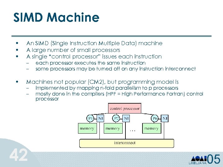SIMD Machine • • • An SIMD (Single Instruction Multiple Data) machine A large number of small processors A single “control processor” issues each instruction • Machines not popular (CM 2), but programming model is – – 42 each processor executes the same instruction some processors may be turned off on any instruction interconnect implemented by mapping n-fold parallelism to p processors mostly done in the compilers (HPF = High Performance Fortran) control processor

Model 4: Hybrid • • Shared memory machines (SMPs) are the fastest commodity machine. Why not build a larger machine by connecting many of them with a network? CLUMP = Cluster of SMPs – – Shared memory within one SMP, message passing outside Clusters, ASCI Red (Intel), . . . Programming model? • • Treat machine as “flat”, always use message passing, even within SMP (simple, but ignore important part of memory hierarchy) Expose two layers: shared memory (Open. MP) and message passing (MPI) higher performance, but ugly to program. 43

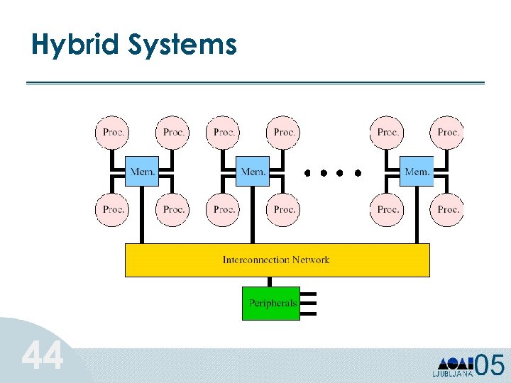Hybrid Systems 44

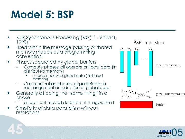Model 5: BSP • • • Bulk Synchronous Processing (BSP) (L. Valiant, 1990) Used within the message passing or shared memory models as a programming convention Phases separated by global barriers – Compute phases: all operate on local data (in distributed memory) • – • • or read access to global data (in shared memory) Communication phases: all participate in rearrangement or reduction of global data Generally all doing the “same thing” in a phase – all do f, but may all do different things within f Simplicity of data parallelism without restrictions 45 BSP superstep

Problem Decomposition q Domain decomposition q Functional decomposition task parallel 46 data parallel

Parallel Programming • directives-based data-parallel language – Such as High Performance Fortran (HPF) or Open. MP – Serial code is made parallel by adding directives (which appear as comments in the serial code) that tell the compiler how to distribute data and work across the processors. – The details of how data distribution, computation, and communications are to be done are left to the compiler. – Usually implemented on shared-memory architectures. • Message Passing (e. g. MPI, PVM) – very flexible approach based on explicit message passing via library calls from standard programming languages – It is left up to the programmer to explicitly divide data and work across the processors as well as manage the communications among them. • Multi-threading in distributed environments 47 – Parallelism is transparent to the programmer – Shared-memory or distributed shared-memory systems

Parallel Programming Issues • The main goal of a parallel program is to get better performance over the serial version. – Performance evaluation • Important issues to take into account: – Load balancing – Minimizing communication – Overlapping communication and computation 48

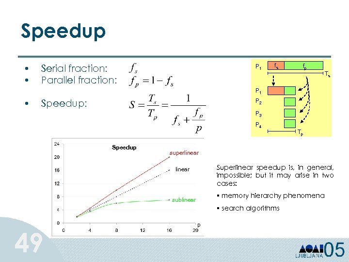Speedup • • Serial fraction: Parallel fraction: P 1 fs fp Ts P 1 • Speedup: P 2 P 3 P 4 Speedup superlinear Superlinear speedup is, in general, impossible; but it may arise in two cases: linear § memory hierarchy phenomena sublinear § search algorithms 49 Tp p

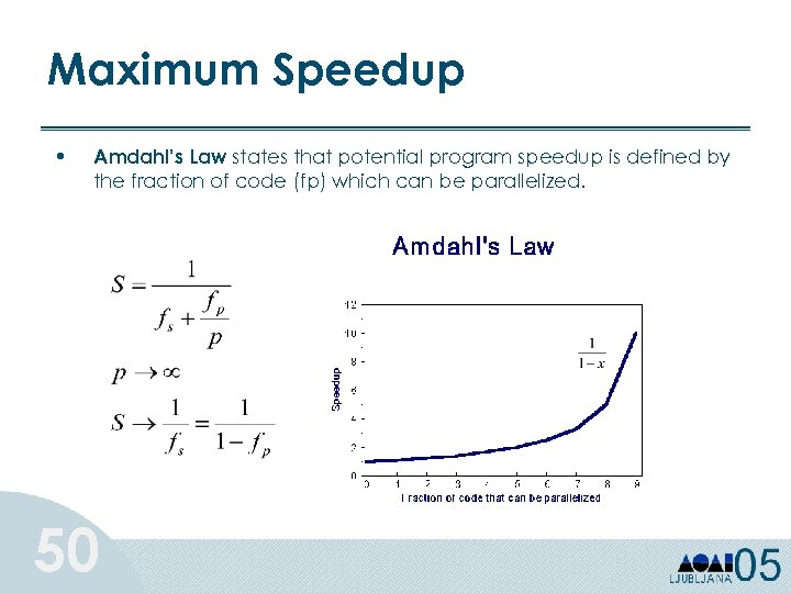Maximum Speedup • Amdahl’s Law states that potential program speedup is defined by the fraction of code (fp) which can be parallelized. 50

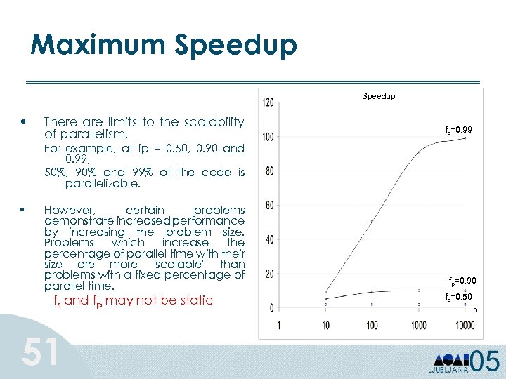Maximum Speedup • There are limits to the scalability of parallelism. fp=0. 99 For example, at fp = 0. 50, 0. 90 and 0. 99, 50%, 90% and 99% of the code is parallelizable. • However, certain problems demonstrate increased performance by increasing the problem size. Problems which increase the percentage of parallel time with their size are more "scalable" than problems with a fixed percentage of parallel time. fs and fp may not be static 51 fp=0. 90 fp=0. 50 p

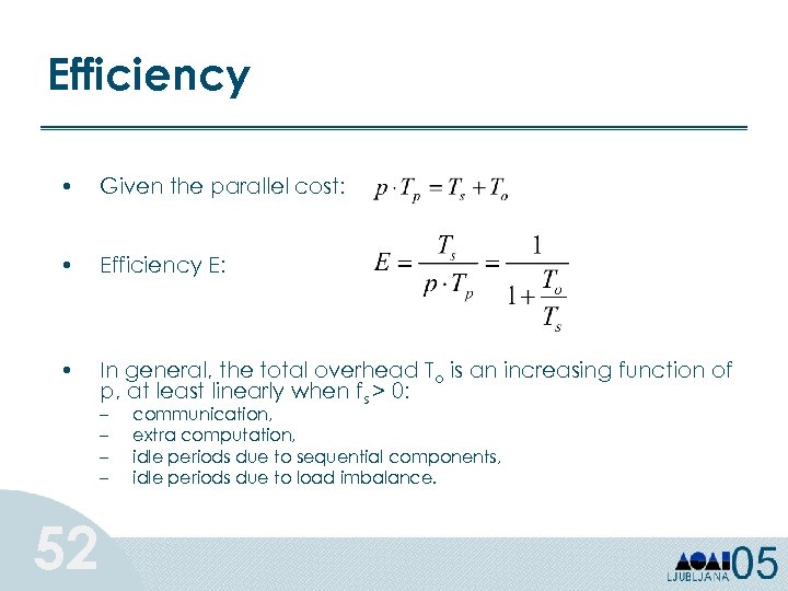Efficiency • Given the parallel cost: • Efficiency E: • In general, the total overhead To is an increasing function of p, at least linearly when fs > 0: – – 52 communication, extra computation, idle periods due to sequential components, idle periods due to load imbalance.

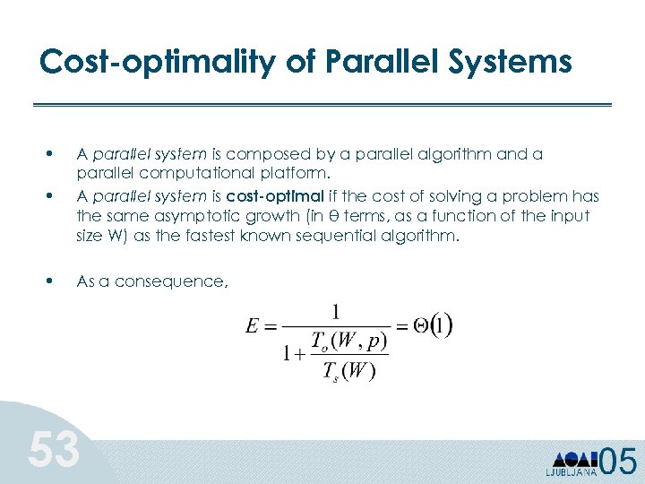Cost-optimality of Parallel Systems • • A parallel system is composed by a parallel algorithm and a parallel computational platform. A parallel system is cost-optimal if the cost of solving a problem has the same asymptotic growth (in θ terms, as a function of the input size W) as the fastest known sequential algorithm. • As a consequence, 53

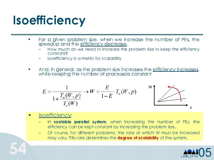Isoefficiency • For a given problem size, when we increase the number of PEs, the speedup and the efficiency decrease. – – • How much do we need to increase the problem size to keep the efficiency constant? Isoefficiency is a metric for scalability And, in general, as the problem size increases the efficiency increases, while keeping the number of processors constant W p • Isoefficiency: – – 54 In scalable parallel system, when increasing the number of PEs, the efficiency can be kept constant by increasing the problem size. Of course, for different problems, the rate at which W must be increased may vary. This rate determines the degree of scalability of the system.

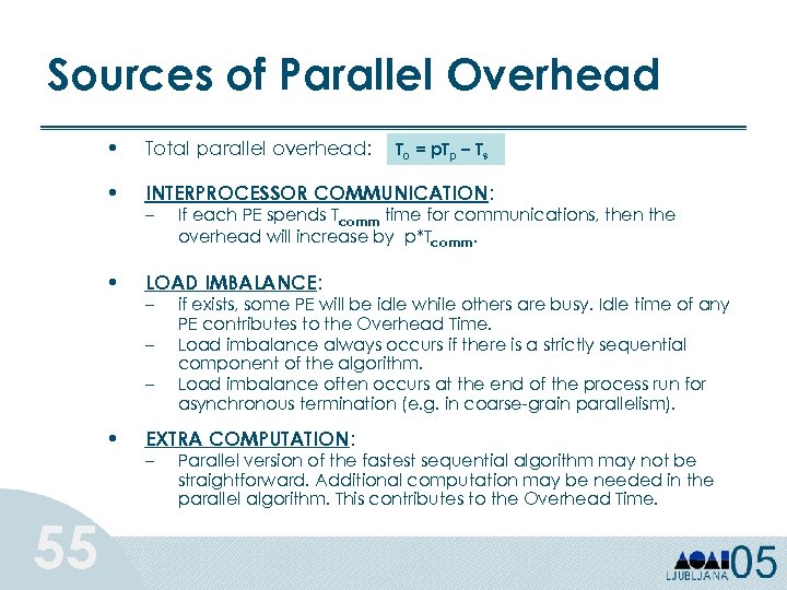Sources of Parallel Overhead • Total parallel overhead: • INTERPROCESSOR COMMUNICATION: • LOAD IMBALANCE: – – • 55 To = p. Tp – Ts If each PE spends Tcomm time for communications, then the overhead will increase by p*Tcomm. if exists, some PE will be idle while others are busy. Idle time of any PE contributes to the Overhead Time. Load imbalance always occurs if there is a strictly sequential component of the algorithm. Load imbalance often occurs at the end of the process run for asynchronous termination (e. g. in coarse-grain parallelism). EXTRA COMPUTATION: – Parallel version of the fastest sequential algorithm may not be straightforward. Additional computation may be needed in the parallel algorithm. This contributes to the Overhead Time.

Load Balancing • Load balancing is the task of equally dividing the work among the available processes. • A range of load balancing problems is determined by – Task costs – Task dependencies – Locality needs • Spectrum of solutions from static to dynamic 56 A closely related problem is scheduling, which determines the order in which tasks run.

Different Load Balancing Problems Load balancing problems differ in: • Tasks costs – Do all tasks have equal costs? – If not, when are the costs known? • Before starting, when task created, or only when task ends • Task dependencies – Can all tasks be run in any order (including parallel)? – If not, when are the dependencies known? • Before starting, when task created, or only when task ends • Locality 57 – Is it important for some tasks to be scheduled on the same processor (or nearby) to reduce communication cost? – When is the information about communication between tasks known?

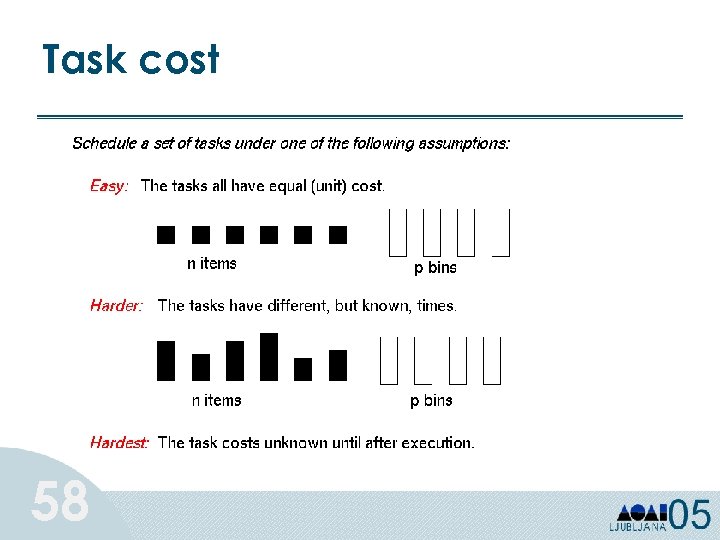Task cost 58

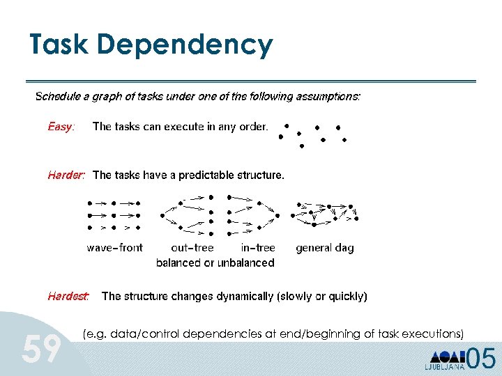Task Dependency 59 (e. g. data/control dependencies at end/beginning of task executions)

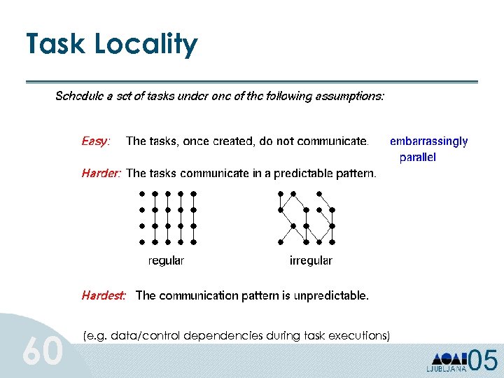Task Locality 60 (e. g. data/control dependencies during task executions)

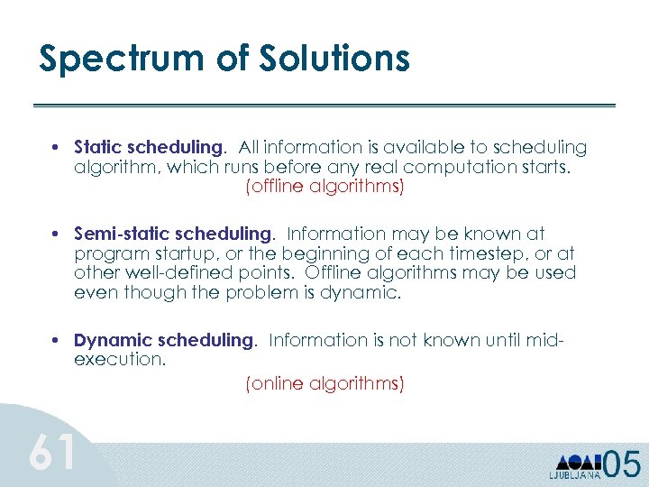Spectrum of Solutions • Static scheduling. All information is available to scheduling algorithm, which runs before any real computation starts. (offline algorithms) • Semi-static scheduling. Information may be known at program startup, or the beginning of each timestep, or at other well-defined points. Offline algorithms may be used even though the problem is dynamic. • Dynamic scheduling. Information is not known until midexecution. (online algorithms) 61

LB Approaches • Static load balancing • Semi-static load balancing • Self-scheduling (manager-workers) • Distributed task queues • Diffusion-based load balancing • DAG scheduling (graph partitioning is NP-complete) • Mixed Parallelism 62

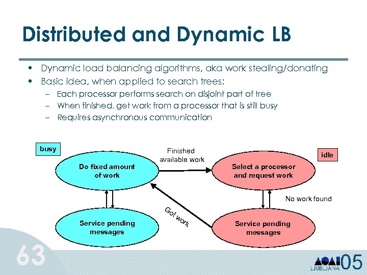Distributed and Dynamic LB • Dynamic load balancing algorithms, aka work stealing/donating • Basic idea, when applied to search trees: – Each processor performs search on disjoint part of tree – When finished, get work from a processor that is still busy – Requires asynchronous communication busy Do fixed amount of work Finished available work idle Select a processor and request work No work found Go Service pending messages 63 tw or k Service pending messages

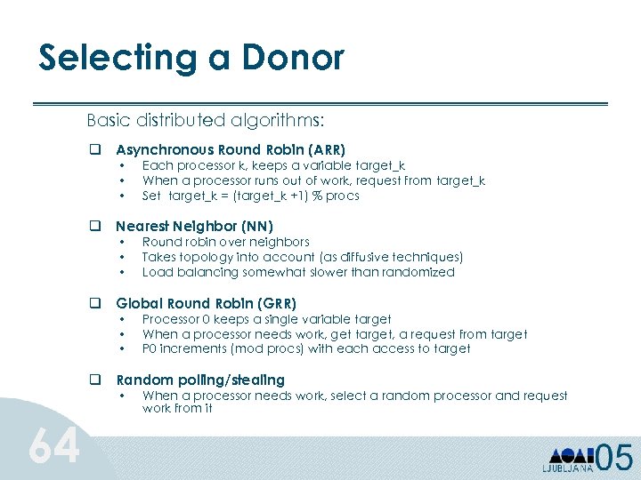Selecting a Donor Basic distributed algorithms: q Asynchronous Round Robin (ARR) • • • Each processor k, keeps a variable target_k When a processor runs out of work, request from target_k Set target_k = (target_k +1) % procs q Nearest Neighbor (NN) • • • Round robin over neighbors Takes topology into account (as diffusive techniques) Load balancing somewhat slower than randomized q Global Round Robin (GRR) • • • Processor 0 keeps a single variable target When a processor needs work, get target, a request from target P 0 increments (mod procs) with each access to target q Random polling/stealing • 64 When a processor needs work, select a random processor and request work from it

Tutorial Outline Ø Part 2: Distributed Data Mining Ø Classification Ø Clustering Ø Association Rules Ø Graph Mining 65

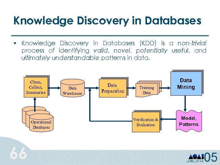Knowledge Discovery in Databases • Knowledge Discovery in Databases (KDD) is a non-trivial process of identifying valid, novel, potentially useful, and ultimately understandable patterns in data. Clean, Collect, Summarize Operational Databases 66 Data Warehouse Data Preparation Training Data Verification & Evaluation Data Mining Model, Patterns

Origins of Data Mining • KDD draws ideas from machine learning/AI, pattern recognition, statistics, database systems, and data visualization. – Prediction Methods Use some variables to predict unknown or future values of other variables. – Description Methods Find human-interpretable patterns that describe the data. • Traditional techniques may be unsuitable 67 – enormity of data – high dimensionality of data – heterogeneous, distributed nature of data

Speeding up Data Mining • Data oriented approach – Discretization – Feature selection – Feature construction (PCA) – Sampling • Methods oriented approach – Efficient and scalable algorithms 68

Speeding up Data Mining • Methods oriented approach (contd. ) – Distributed and parallel data-mining • Task or control parallelism • Data parallelism • Hybrid parallelism – Distributed-data mining • Voting • Meta-learning, etc. 69

Tutorial Outline Ø Part 2: Distributed Data Mining Ø Classification Ø Clustering Ø Association Rules Ø Graph Mining 70

What is Classification? Classification is the process of assigning new objects to predefined categories or classes • Given a set of labeled records • Build a model (e. g. a decision tree) • Predict labels for future unlabeled records 71

Classification learning • Supervised learning (labels are known) • Example described in terms of attributes – Categorical (unordered symbolic values) – Numeric (integers, reals) • Class (output/predicted attribute): – categorical for classification – numeric for regression 72

Classification learning • Training set: – set of examples, where each example is a feature vector (i. e. , a set of pairs) with its associated class. The model is built on this set. • Test set: – a set of examples disjoint from the training set, used for testing the accuracy of a model. 73

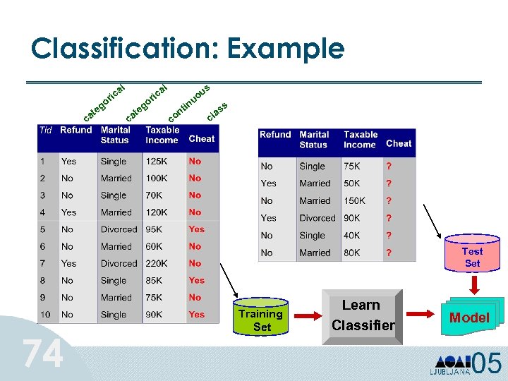Classification: Example al al ric go te ca s ric go c e at i u uo n c t on ss a cl Test Set 74 Training Set Learn Classifier Model

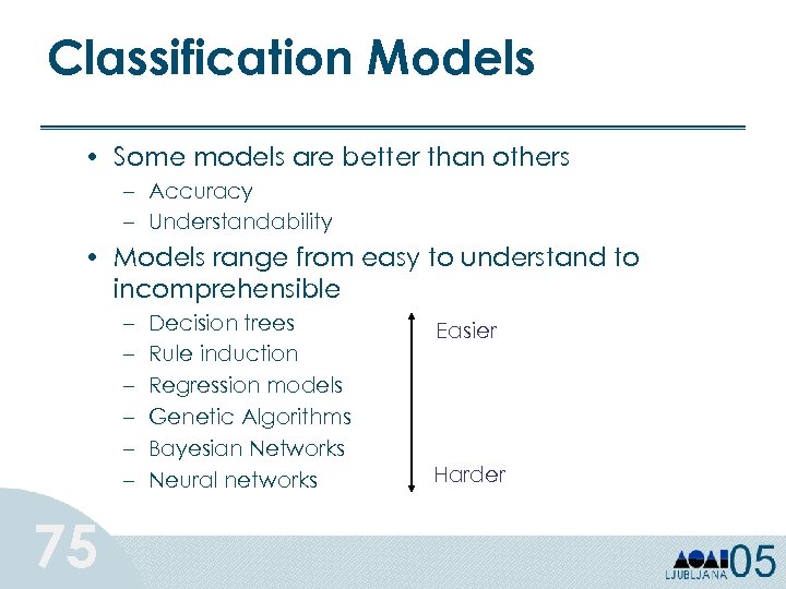Classification Models • Some models are better than others – Accuracy – Understandability • Models range from easy to understand to incomprehensible – – – 75 Decision trees Rule induction Regression models Genetic Algorithms Bayesian Networks Neural networks Easier Harder

Decision Trees • Decision tree models are better suited for data mining: – – 76 Inexpensive to construct Easy to Interpret Easy to integrate with database systems Comparable or better accuracy in many applications

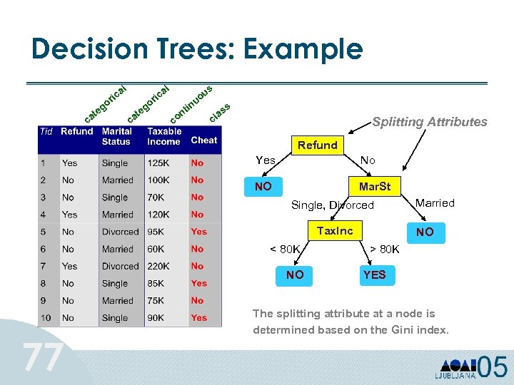Decision Trees: Example al al ric go te ca s ric go c e at i u uo n c t on ss a cl Splitting Attributes Refund Yes No NO Mar. St Single, Divorced Tax. Inc < 80 K NO 77 Married NO > 80 K YES The splitting attribute at a node is determined based on the Gini index.

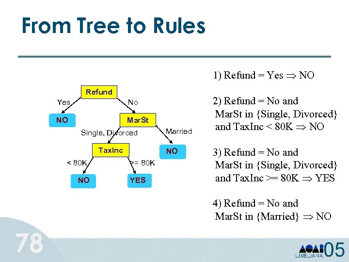From Tree to Rules 1) Refund = Yes NO Refund Yes No NO Mar. St Single, Divorced Tax. Inc < 80 K NO Married NO >= 80 K YES 2) Refund = No and Mar. St in {Single, Divorced} and Tax. Inc < 80 K NO 3) Refund = No and Mar. St in {Single, Divorced} and Tax. Inc >= 80 K YES 4) Refund = No and Mar. St in {Married} NO 78

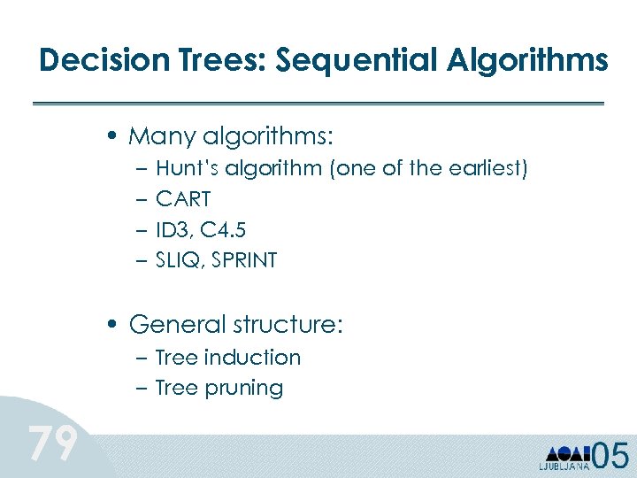Decision Trees: Sequential Algorithms • Many algorithms: – – Hunt’s algorithm (one of the earliest) CART ID 3, C 4. 5 SLIQ, SPRINT • General structure: – Tree induction – Tree pruning 79

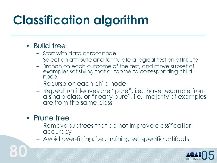Classification algorithm • Build tree – Start with data at root node – Select an attribute and formulate a logical test on attribute – Branch on each outcome of the test, and move subset of examples satisfying that outcome to corresponding child node – Recurse on each child node – Repeat until leaves are “pure”, i. e. , have example from a single class, or “nearly pure”, i. e. , majority of examples are from the same class • Prune tree 80 – Remove subtrees that do not improve classification accuracy – Avoid over-fitting, i. e. , training set specific artifacts

Build tree • Evaluate split-points for all attributes • Select the “best” point and the “winning” attribute • Split the data into two • Breadth/depth-first construction • CRITICAL STEPS: – Formulation of good split tests – Selection measure for attributes 81

How to capture good splits? • Occam’s razor: Prefer the simplest hypothesis that fits the data • Minimum message/description length – – dataset D hypotheses H 1, H 2, …, Hx describing D MML(Hi) = Mlength(Hi)+Mlength(D|Hi) pick Hk with minimum MML • Mlength given by Gini index, Gain, etc. 82

Tree pruning using MDL • Data encoding: sum classification errors • Model encoding: – Encode the tree structure – Encode the split points • Pruning: choose smallest length option – Convert to leaf – Prune left or right child – Do nothing 83

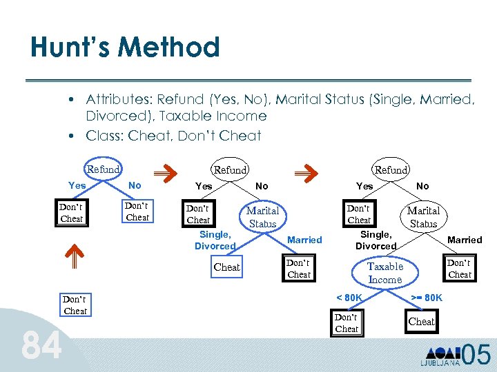Hunt’s Method • Attributes: Refund (Yes, No), Marital Status (Single, Married, Divorced), Taxable Income • Class: Cheat, Don’t Cheat Refund Yes Don’t Cheat Refund No Don’t Cheat Yes No Don’t Cheat Single, Divorced Cheat Don’t Cheat 84 Refund Yes Don’t Cheat Marital Status Married Single, Divorced Don’t Cheat No Marital Status Married Don’t Cheat Taxable Income < 80 K >= 80 K Don’t Cheat

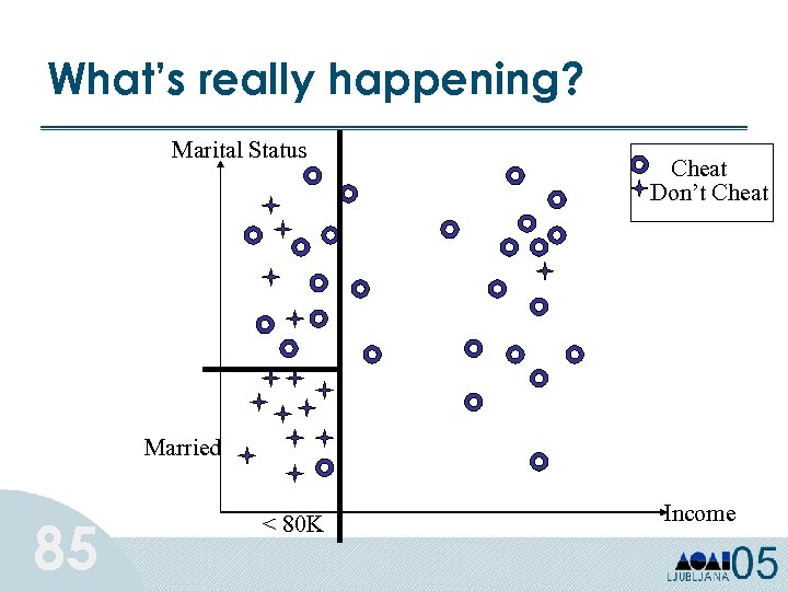What’s really happening? Marital Status Cheat Don’t Cheat Married 85 < 80 K Income

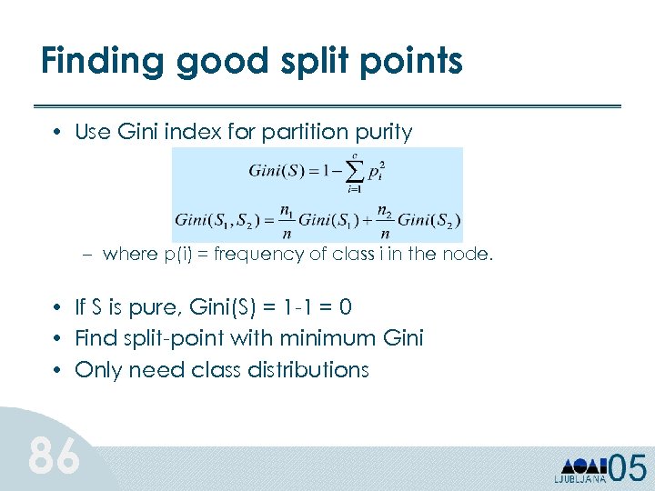Finding good split points • Use Gini index for partition purity – where p(i) = frequency of class i in the node. • If S is pure, Gini(S) = 1 -1 = 0 • Find split-point with minimum Gini • Only need class distributions 86

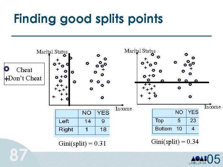Finding good splits points Marital Status Cheat Don’t Cheat Income 87 Gini(split) = 0. 31 Gini(split) = 0. 34

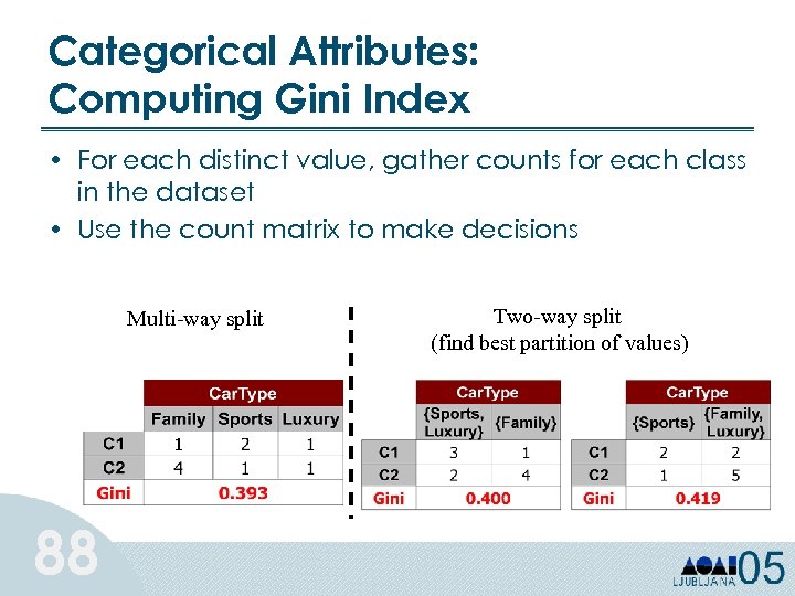Categorical Attributes: Computing Gini Index • For each distinct value, gather counts for each class in the dataset • Use the count matrix to make decisions Multi-way split 88 Two-way split (find best partition of values)

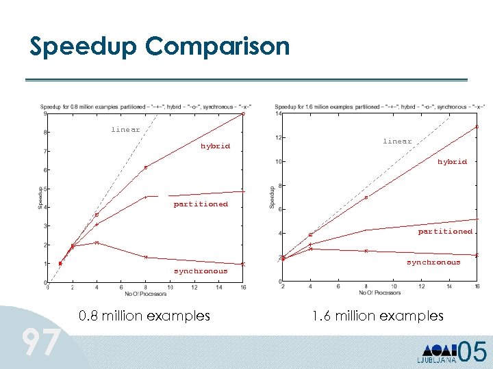
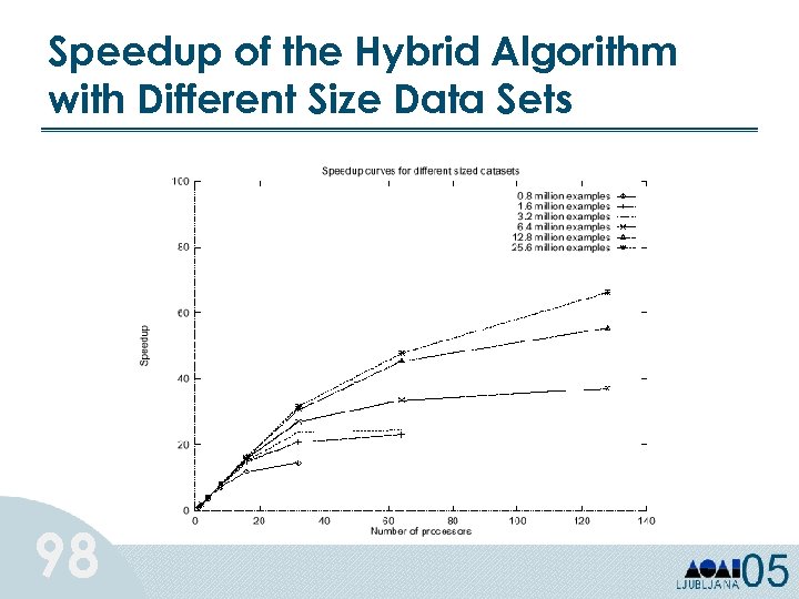
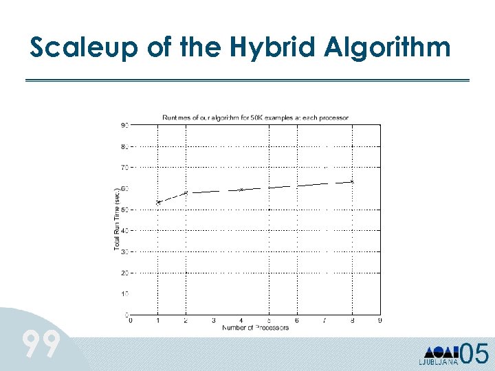
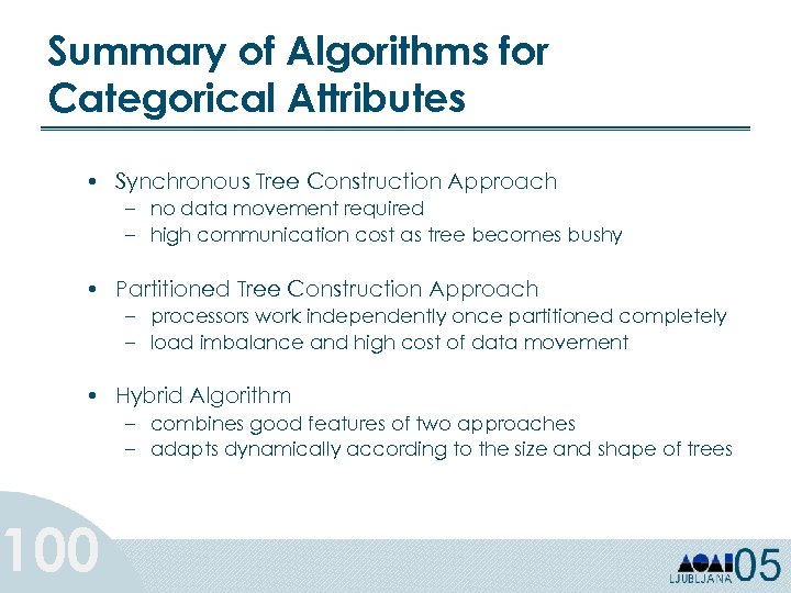
Decision Trees: Parallel Algorithms Approaches for Categorical Attributes: • Synchronous Tree Construction (data parallel) – no data movement required – high communication cost as tree becomes bushy • Partitioned Tree Construction (task parallel) – processors work independently once partitioned completely – load imbalance and high cost of data movement • Hybrid Algorithm – combines good features of two approaches – adapts dynamically according to the size and shape of trees 89

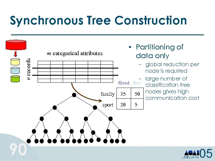Synchronous Tree Construction n records m categorical attributes 90 • Partitioning of data only – global reduction per node is required – large number of Good Bad classification tree family 35 50 nodes gives high communication cost sport 20 5

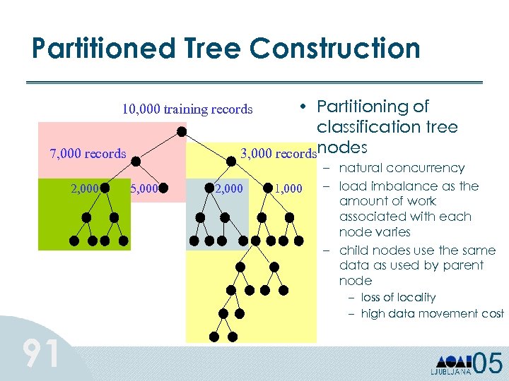Partitioned Tree Construction • Partitioning of classification tree 3, 000 recordsnodes 10, 000 training records 7, 000 records 2, 000 5, 000 2, 000 1, 000 – natural concurrency – load imbalance as the amount of work associated with each node varies – child nodes use the same data as used by parent node – loss of locality – high data movement cost 91

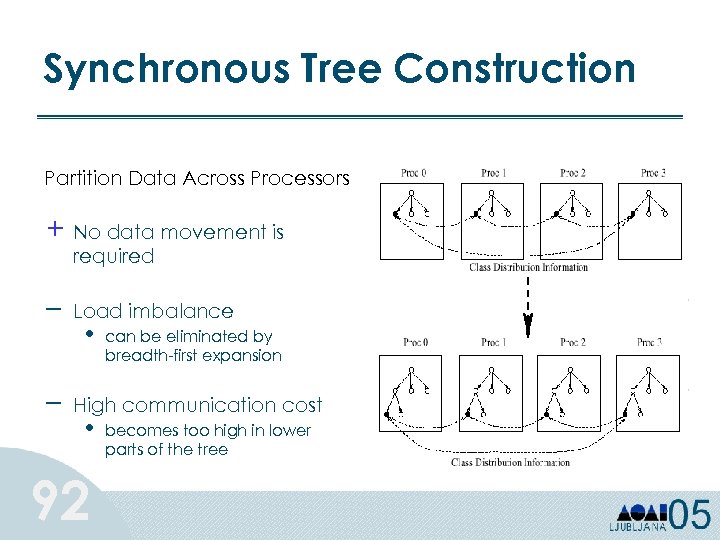Synchronous Tree Construction Partition Data Across Processors + No data movement is required – – Load imbalance • can be eliminated by breadth-first expansion High communication cost • 92 becomes too high in lower parts of the tree

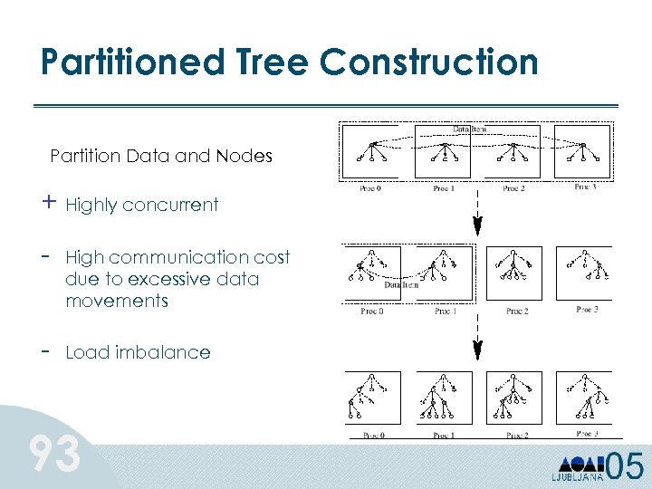Partitioned Tree Construction Partition Data and Nodes + Highly concurrent - High communication cost due to excessive data movements Load imbalance 93

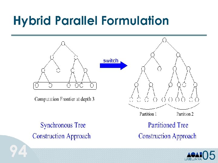Hybrid Parallel Formulation switch 94

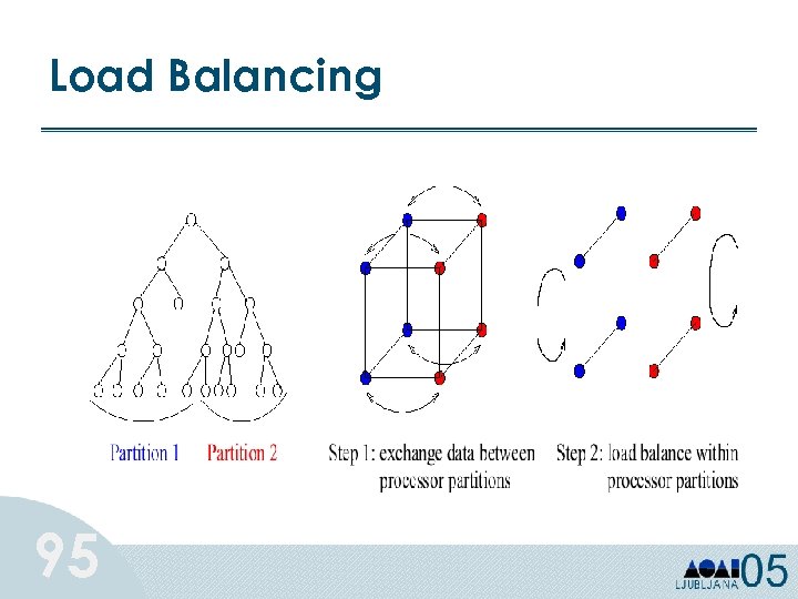Load Balancing 95

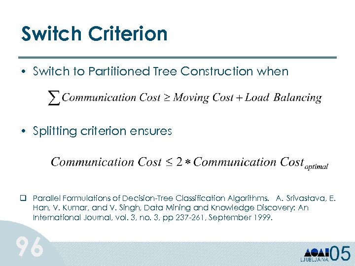Switch Criterion • Switch to Partitioned Tree Construction when • Splitting criterion ensures q Parallel Formulations of Decision-Tree Classification Algorithms. A. Srivastava, E. Han, V. Kumar, and V. Singh, Data Mining and Knowledge Discovery: An International Journal, vol. 3, no. 3, pp 237 -261, September 1999. 96

Speedup Comparison linear hybrid partitioned synchronous 97 0. 8 million examples synchronous 1. 6 million examples

Speedup of the Hybrid Algorithm with Different Size Data Sets 98

Scaleup of the Hybrid Algorithm 99

Summary of Algorithms for Categorical Attributes • Synchronous Tree Construction Approach – no data movement required – high communication cost as tree becomes bushy • Partitioned Tree Construction Approach – processors work independently once partitioned completely – load imbalance and high cost of data movement • Hybrid Algorithm 100 – combines good features of two approaches – adapts dynamically according to the size and shape of trees

Tutorial Outline 101 Ø Part 2: Distributed Data Mining Ø Classification Ø Clustering Ø Association Rules Ø Graph Mining

Clustering: Definition • Given a set of data points, each having a set of attributes, and a similarity measure among them, find clusters such that – Data points in one cluster are more similar to one another – Data points in separate clusters are less similar to one another 102

Clustering Given N k-dimensional feature vectors, find a “meaningful” partition of the N examples into c subsets or groups. – Discover the “labels” automatically – c may be given, or “discovered” Much more difficult than classification, since in the latter the groups are given, and we seek a compact description. 103

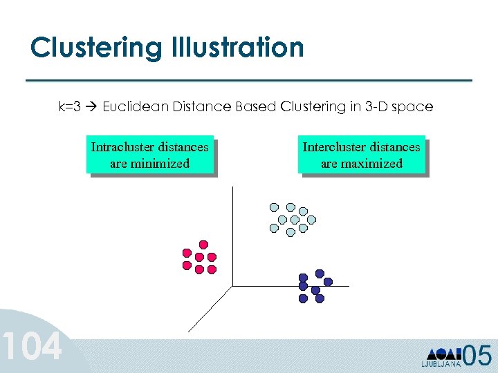Clustering Illustration k=3 Euclidean Distance Based Clustering in 3 -D space 104 Intracluster distances are minimized Intercluster distances are maximized

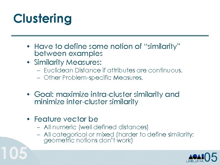Clustering • Have to define some notion of “similarity” between examples • Similarity Measures: – Euclidean Distance if attributes are continuous. – Other Problem-specific Measures. • Goal: maximize intra-cluster similarity and minimize inter-cluster similarity • Feature vector be 105 – All numeric (well defined distances) – All categorical or mixed (harder to define similarity; geometric notions don’t work)

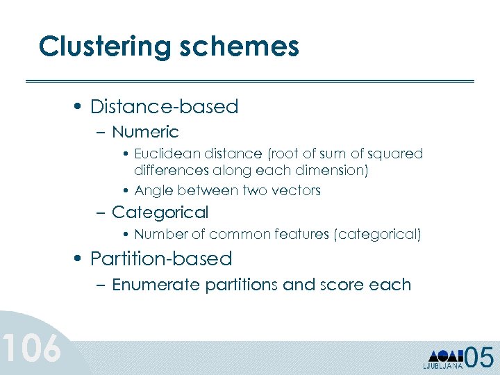Clustering schemes 106 • Distance-based – Numeric • Euclidean distance (root of sum of squared differences along each dimension) • Angle between two vectors – Categorical • Number of common features (categorical) • Partition-based – Enumerate partitions and score each

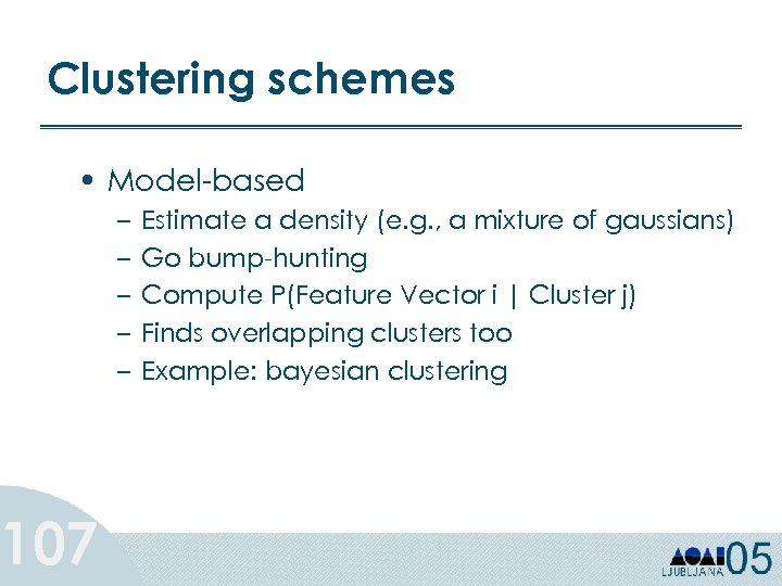Clustering schemes • Model-based 107 – – – Estimate a density (e. g. , a mixture of gaussians) Go bump-hunting Compute P(Feature Vector i | Cluster j) Finds overlapping clusters too Example: bayesian clustering

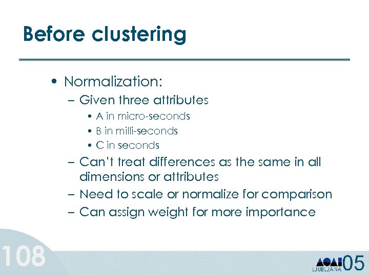Before clustering 108 • Normalization: – Given three attributes • A in micro-seconds • B in milli-seconds • C in seconds – Can’t treat differences as the same in all dimensions or attributes – Need to scale or normalize for comparison – Can assign weight for more importance

The k-means algorithm • Specify ‘k’, the number of clusters • Guess ‘k’ seed cluster centers • 1) Look at each example and assign it to the center that is closest • 2) Recalculate the center • Iterate on steps 1 and 2 till centers converge or for a fixed number of times 109

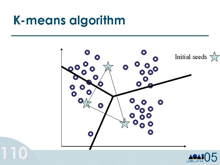K-means algorithm 110 Initial seeds

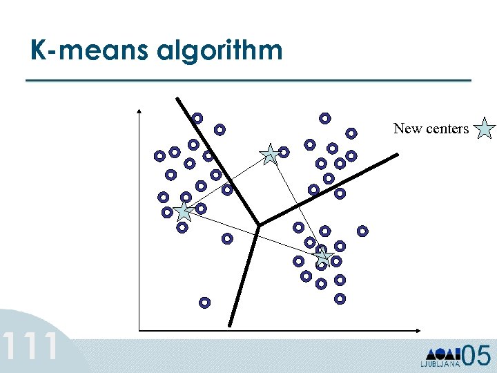K-means algorithm 111 New centers

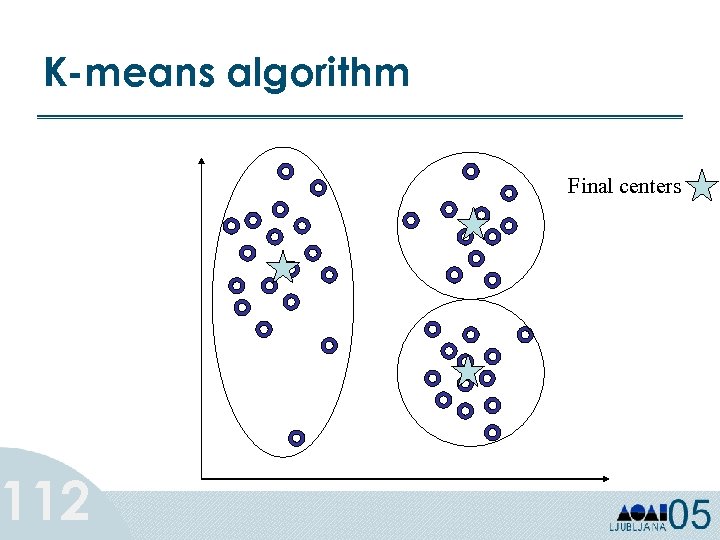K-means algorithm 112 Final centers

Operations in k-means • Main Operation: Calculate distance to all k means or centroids • Other operations: 113 – Find the closest centroid for each point – Calculate mean squared error (MSE) for all points – Recalculate centroids

Parallel k-means 114 • Divide N points among P processors • Replicate the k centroids • Each processor computes distance of each local point to the centroids • Assign points to closest centroid and compute local MSE • Perform reduction for global centroids and global MSE value

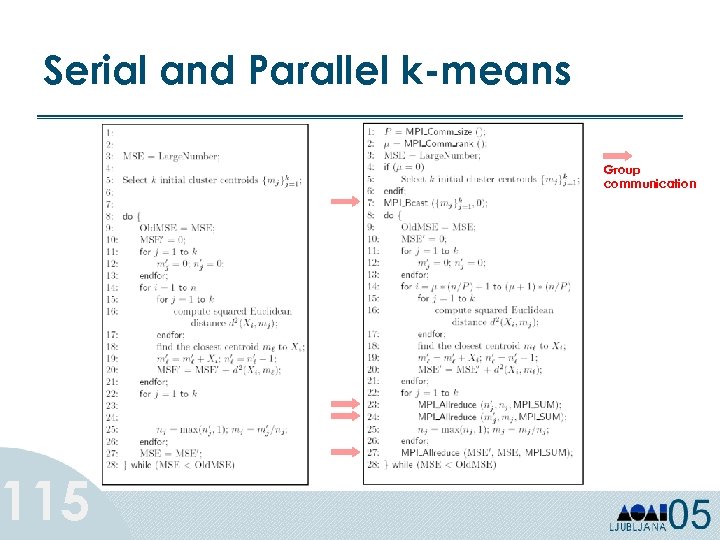Serial and Parallel k-means 115 Group communication

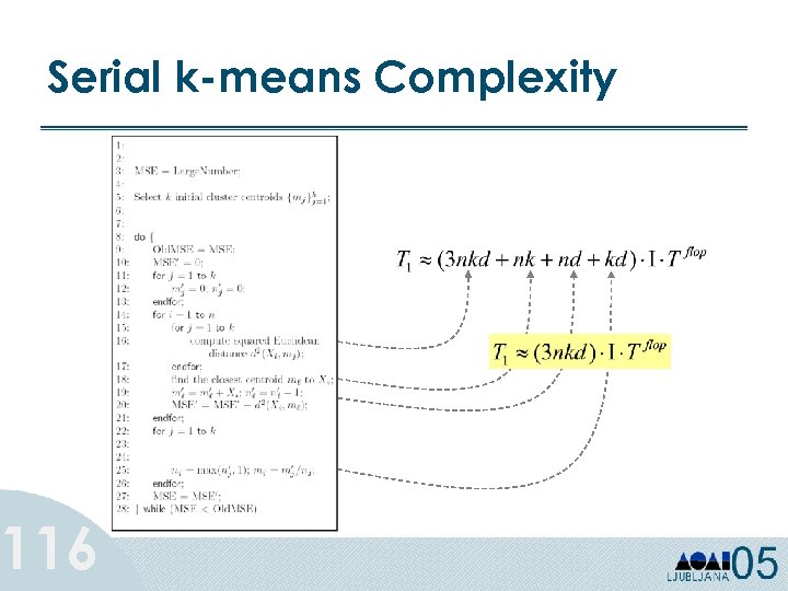Serial k-means Complexity 116

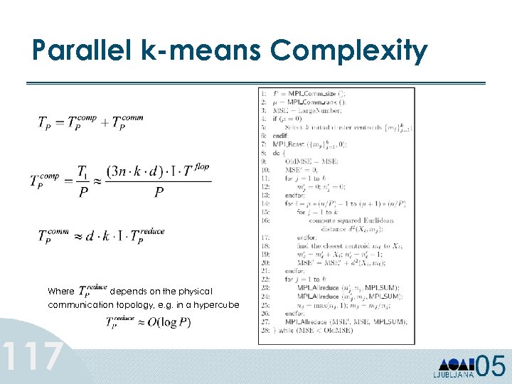Parallel k-means Complexity Where depends on the physical communication topology, e. g. in a hypercube 117

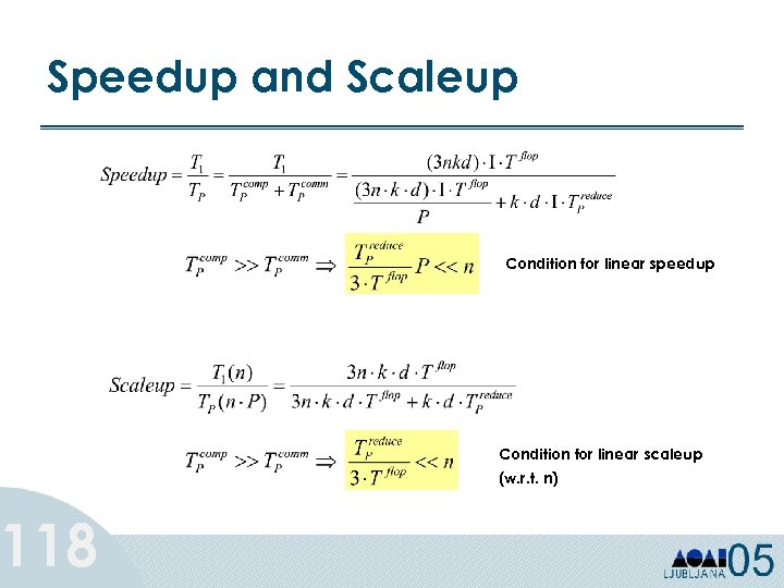Speedup and Scaleup 118 Condition for linear speedup Condition for linear scaleup (w. r. t. n)

Tutorial Outline 119 Ø Part 2: Distributed Data Mining Ø Classification Ø Clustering Ø Association Rules § Frequent Itemset Mining Ø Graph Mining

ARM: Definition • Given a set of records each of which contain some number of items from a given collection; – Produce dependency rules which will predict occurrence of an item based on occurrences of other items. 120

ARM Definition • Given a set of items/attributes, and a set of objects containing a subset of the items • Find rules: if I 1 then I 2 (sup, conf) • I 1, I 2 are sets of items • I 1, I 2 have sufficient support: P(I 1+I 2) • Rule has sufficient confidence: P(I 2|I 1) 121

Association Mining 122 • User specifies “interestingness” – Minimum support (minsup) – Minimum confidence (minconf) • Find all frequent itemsets (> minsup) – Exponential Search Space – Computation and I/O Intensive • Generate strong rules (> minconf) – Relatively cheap

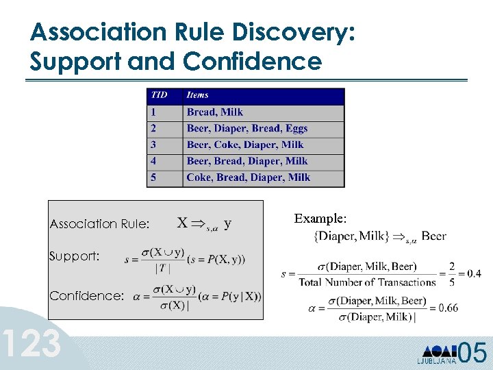Association Rule Discovery: Support and Confidence Association Rule: Support: Confidence: 123 Example:

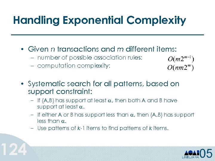Handling Exponential Complexity • Given n transactions and m different items: – number of possible association rules: – computation complexity: • Systematic search for all patterns, based on support constraint: 124 – If {A, B} has support at least a, then both A and B have support at least a. – If either A or B has support less than a, then {A, B} has support less than a. – Use patterns of k-1 items to find patterns of k items.

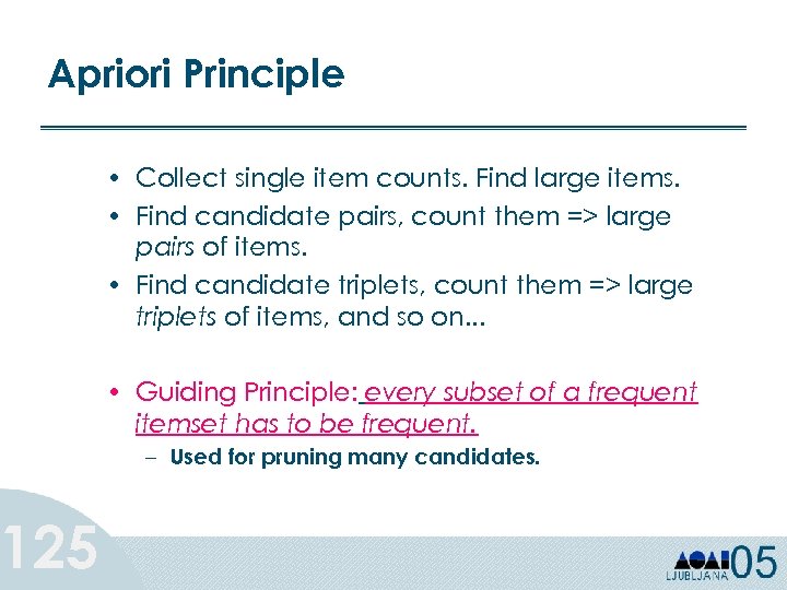Apriori Principle 125 • Collect single item counts. Find large items. • Find candidate pairs, count them => large pairs of items. • Find candidate triplets, count them => large triplets of items, and so on. . . • Guiding Principle: every subset of a frequent itemset has to be frequent. – Used for pruning many candidates.

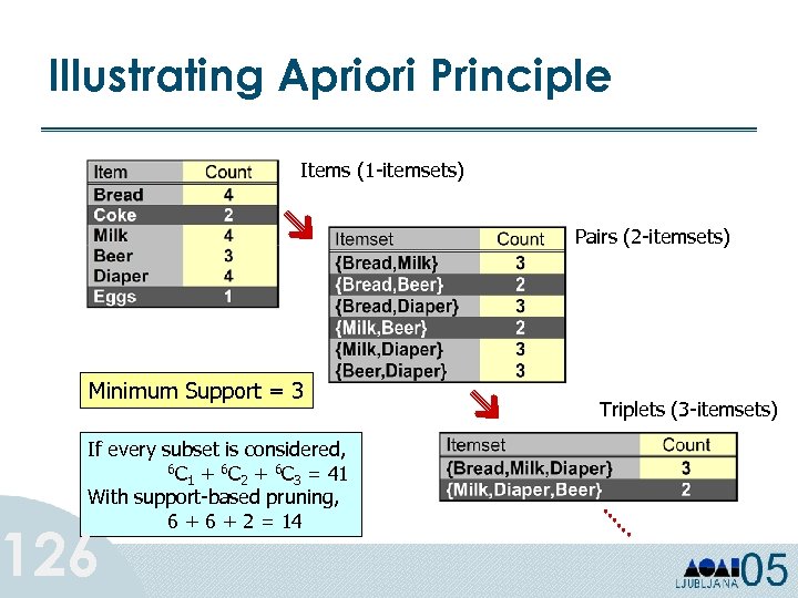Illustrating Apriori Principle Items (1 -itemsets) Pairs (2 -itemsets) Minimum Support = 3 If every subset is considered, 6 C + 6 C = 41 1 2 3 With support-based pruning, 6 + 2 = 14 126 Triplets (3 -itemsets)

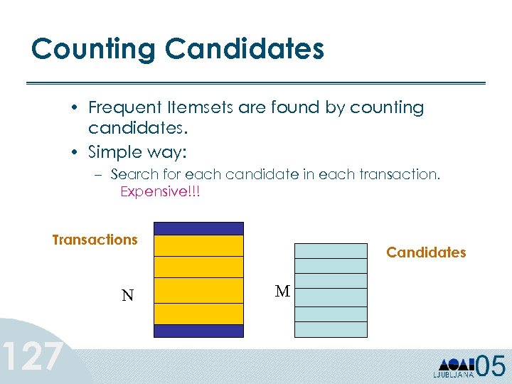Counting Candidates • Frequent Itemsets are found by counting candidates. • Simple way: – Search for each candidate in each transaction. Expensive!!! Transactions 127 N Candidates M

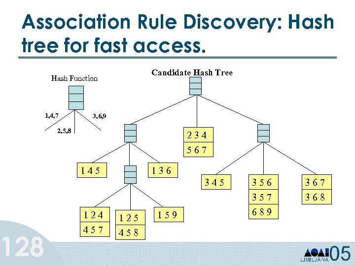Association Rule Discovery: Hash tree for fast access. 128 Candidate Hash Tree Hash Function 1, 4, 7 3, 6, 9 2, 5, 8 234 567 145 136 345 124 125 457 458 159 356 357 689 367 368

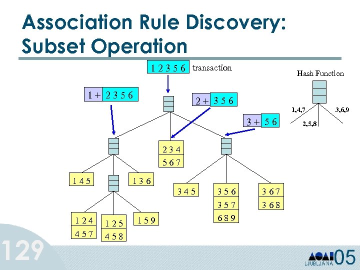Association Rule Discovery: Subset Operation 129 1 2 3 5 6 transaction 1+ 2356 Hash Function 2+ 356 1, 4, 7 3+ 56 234 567 145 136 345 124 457 125 458 159 356 357 689 367 368 2, 5, 8 3, 6, 9

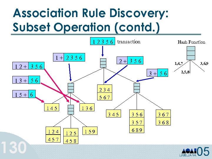Association Rule Discovery: Subset Operation (contd. ) 1 2 3 5 6 transaction 1+ 2356 Hash Function 2+ 356 1, 4, 7 3+ 56 13+ 56 234 567 15+ 6 130 145 136 345 124 457 125 458 159 356 357 689 367 368 2, 5, 8 3, 6, 9

Parallel Formulation of Association Rules • Large-scale problems have: – Huge Transaction Datasets (10 s of TB) – Large Number of Candidates. • Parallel Approaches: 131 – Partition the Transaction Database, or – Partition the Candidates, or – Both

Parallel Association Rules: Count Distribution (CD) 132 • Each Processor has complete candidate hash tree. • Each Processor updates its hash tree with local data. • Each Processor participates in global reduction to get global counts of candidates in the hash tree. • Multiple database scans per iteration are required if hash tree too big for memory.

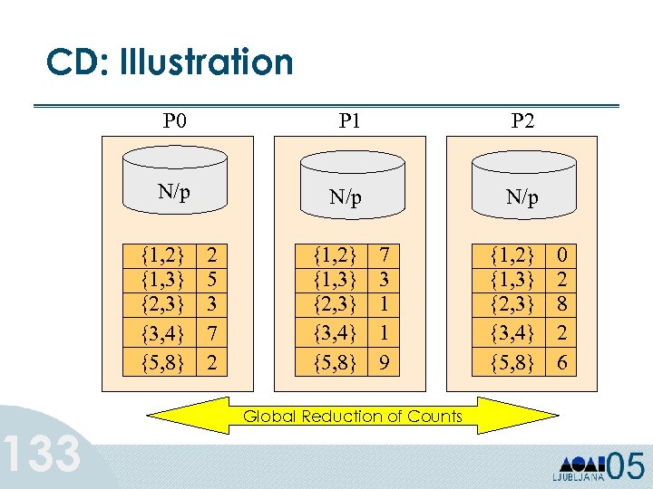CD: Illustration 133 P 0 P 1 P 2 N/p N/p {1, 2} {1, 3} {2, 3} {3, 4} {5, 8} 2 5 3 7 2 {1, 2} {1, 3} {2, 3} {3, 4} {5, 8} 7 3 1 1 9 Global Reduction of Counts {1, 2} {1, 3} {2, 3} {3, 4} {5, 8} 0 2 8 2 6

Parallel Association Rules: Data Distribution (DD) 134 • Candidate set is partitioned among the processors. • Once local data has been partitioned, it is broadcast to all other processors. • High Communication Cost due to data movement. • Redundant work due to multiple traversals of the hash trees.

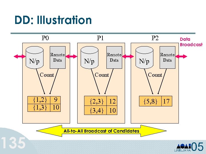DD: Illustration 135 P 0 N/p P 1 Remote Data N/p P 2 Remote Data N/p Data Broadcast Remote Data Count {1, 2} 9 {1, 3} 10 {2, 3} 12 {3, 4} 10 {5, 8} 17 All-to-All Broadcast of Candidates

Parallel Association Rules: Intelligent Data Distribution (IDD) 136 • Data Distribution using point-to-point communication. • Intelligent partitioning of candidate sets. – Partitioning based on the first item of candidates. – Bitmap to keep track of local candidate items. • Pruning at the root of candidate hash tree using the bitmap. • Suitable for single data source such as database server. • With smaller candidate set, load balancing is difficult.

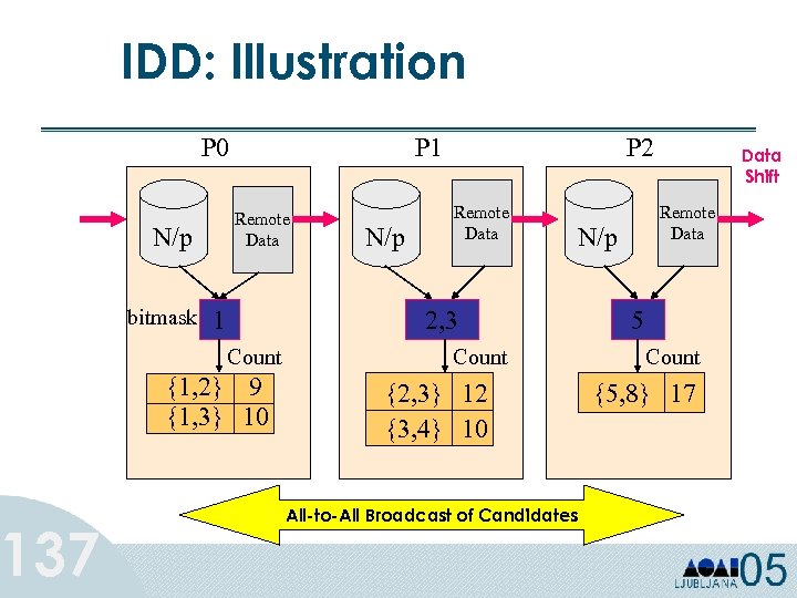137 IDD: Illustration P 0 Remote Data N/p bitmask P 1 1 N/p P 2 Remote Data 2, 3 Count {1, 2} 9 {1, 3} 10 Count {2, 3} 12 {3, 4} 10 All-to-All Broadcast of Candidates Data Shift Remote Data N/p 5 Count {5, 8} 17

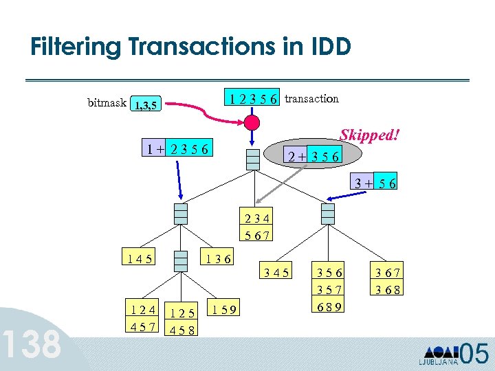Filtering Transactions in IDD 138 1 2 3 5 6 transaction bitmask 1, 3, 5 Skipped! 1+ 2356 2+ 356 3+ 56 234 567 145 124 457 136 125 458 159 345 356 357 689 367 368

Parallel Association Rules: Hybrid Distribution (HD) • Candidate set is partitioned into G groups to just fit in main memory – Ensures Good load balance with smaller candidate set. • Logical processor mesh G x P/G is formed. • Perform IDD along the column processors – Data movement among processors is minimized. • Perform CD along the row processors – Smaller number of processors in global reduction operation. 139

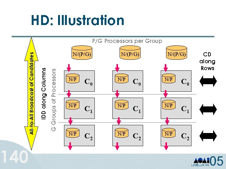140 HD: Illustration G Groups of Processors N/(P/G) IDD along Columns All-to-All Broadcast of Candidates P/G Processors per Group N/(P/G) N/P C 0 N/P C 1 N/P C 2 CD along Rows

Parallel Association Rules: Comments • HD has shown the same linear speedup and sizeup behavior as that of CD. • HD exploits total aggregate main memory, while CD does not. • IDD has much better scaleup behavior than DD. 141

Tutorial Outline 142 Ø Part 2: Distributed Data Mining Ø Classification Ø Clustering Ø Association Rules Ø Graph Mining § Frequent Subgraph Mining

Graph Mining 143 Market Basket Analysis Association Rule Mining (ARM) find frequent itemset • Search space: – – – • Unstructured data: only item type is important item set I, |I|=n power set P(I), |P(I)| = 2 n pruning technique to make the search feasible Subset test: – for each user transaction t and each candidate frequent-itemset s we need a subset test in order to compute the support (frequency). Molecular Compound Analysis Frequent Subgraph Mining (FSM) find frequent subgraph • Bigger search space: – • Structured data: atom types are not sufficient; atoms have bonds with other atoms. Subgraph isomorphism test: – – for each graph and each candidate frequent-subgraph we need a subgraph isomorphism test. N. B. : for general graphs the subgraph isomorphism test is NP-complete

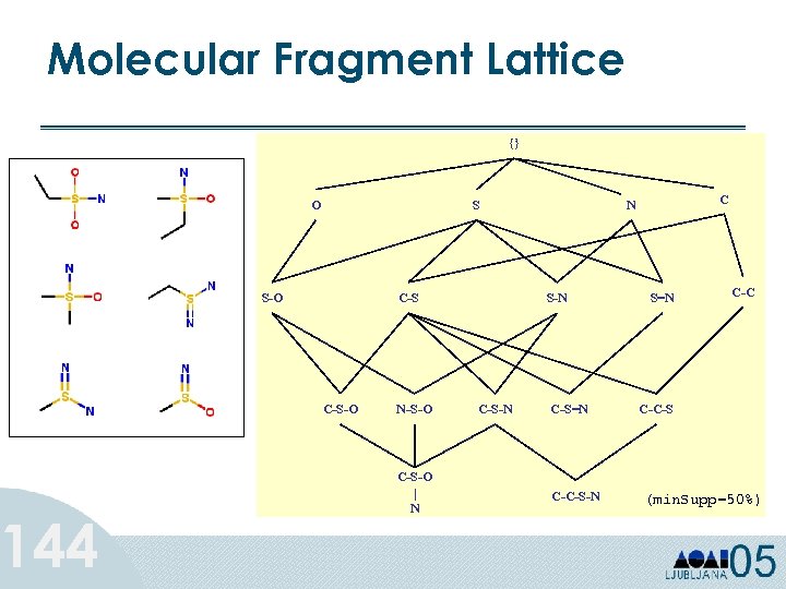Molecular Fragment Lattice 144 {} O S S-O C-S-O N-S-O C-S-O | N S-N C-S-N C N C-S=N C-C-S-N S=N C-C-S (min. Supp=50%)

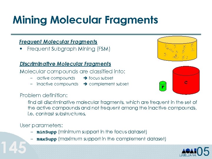Mining Molecular Fragments Frequent Molecular Fragments • Frequent Subgraph Mining (FSM) Discriminative Molecular Fragments Molecular compounds are classified into: – – active compounds inactive compounds focus subset complement subset F C Problem definition: find all discriminative molecular fragments, which are frequent in the set of the active compounds and not frequent among the inactive compounds, i. e. contrast substructures. User parameters: 145 – min. Supp (minimum support in the focus dataset) – max. Supp (maximum support in the complement dataset)

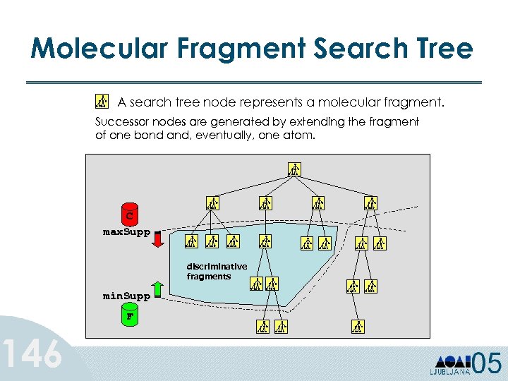Molecular Fragment Search Tree 146 A search tree node represents a molecular fragment. Successor nodes are generated by extending the fragment of one bond and, eventually, one atom. C max. Supp discriminative fragments min. Supp F

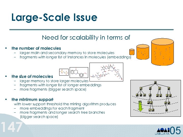Large-Scale Issue Need for scalability in terms of • the number of molecules • the size of molecules • the minimum support – – – larger main and secondary memory to store molecules fragments with longer list of instances in molecules (embeddings) larger memory to store larger molecules fragments with longer list of longer embeddings more fragments (bigger search space) with lower support threshold the mining algorithm produces – more embeddings for each fragment – more fragments and longer search tree branches (bigger search space) 147

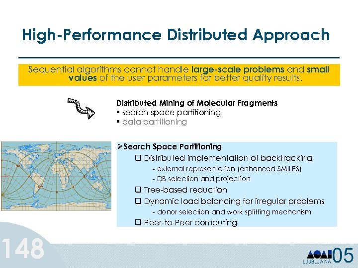High-Performance Distributed Approach Sequential algorithms cannot handle large-scale problems and small values of the user parameters for better quality results. 148 Distributed Mining of Molecular Fragments § search space partitioning § data partitioning ØSearch Space Partitioning q Distributed implementation of backtracking - external representation (enhanced SMILES) - DB selection and projection q Tree-based reduction q Dynamic load balancing for irregular problems - donor selection and work splitting mechanism q Peer-to-Peer computing

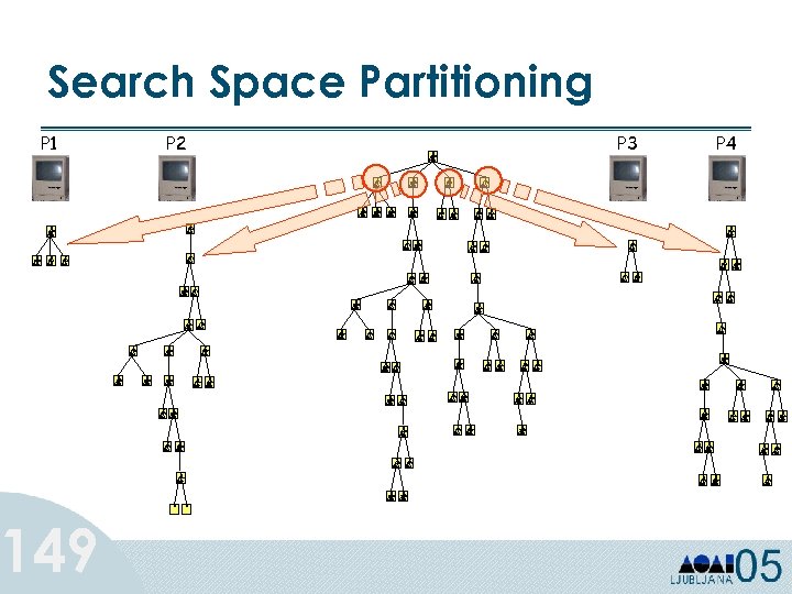Search Space Partitioning P 1 149 P 2 P 3 P 4

Search Space Partitioning q 4 th kind of search-tree pruning: “Distributed Computing pruning” § prune a search node, generate a new job and assign it to an idle processor q asynchronous communication and low overhead 150 § backtracking is particularly suitable to parallel processing because a subtree rooted at any node can be searched independently

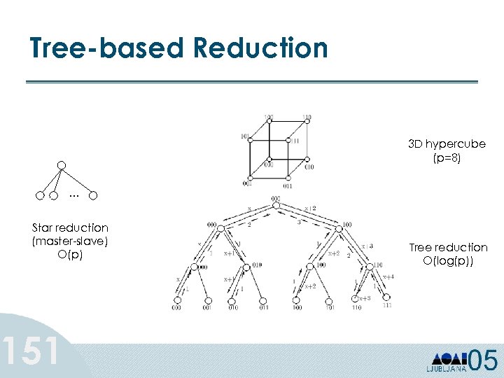Tree-based Reduction 3 D hypercube (p=8) … Star reduction (master-slave) O(p) 151 Tree reduction O(log(p))

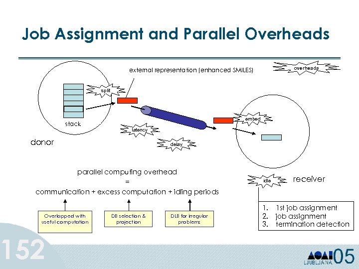Job Assignment and Parallel Overheads overheads external representation (enhanced SMILES) split stack embed latency donor delay parallel computing overhead = communication + excess computation + idling periods Overlapped with useful computation 152 DB selection & projection DLB for irregular problems idle 1. 2. 3. receiver 1 st job assignment termination detection

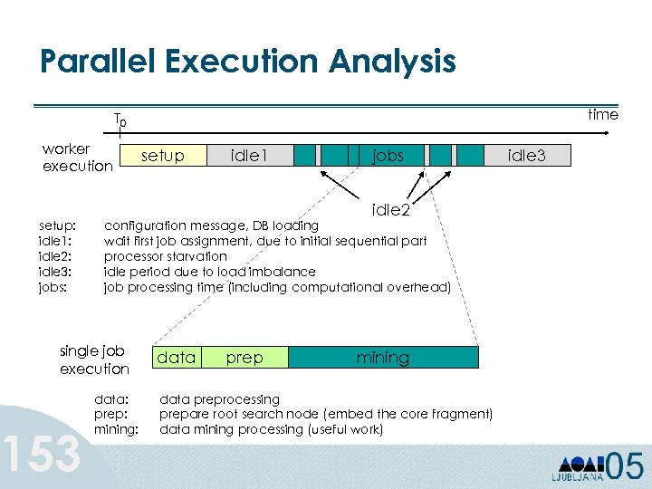Parallel Execution Analysis time T 0 worker execution setup: idle 1: idle 2: idle 3: jobs: idle 1 jobs idle 2 configuration message, DB loading wait first job assignment, due to initial sequential part processor starvation idle period due to load imbalance job processing time (including computational overhead) single job execution 153 setup data: prep: mining: data prep mining data preprocessing prepare root search node (embed the core fragment) data mining processing (useful work) idle 3

Load Balancing 154 The search space is not know a priori and is very irregular q Dynamic load balancing § receiver-initiated approach - donor selection - work splitting mechanism The DLB determines the overall performance and efficiency.

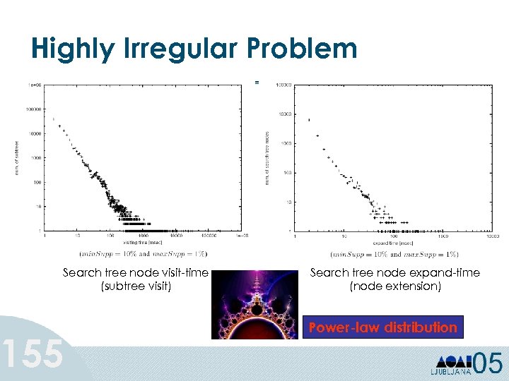Highly Irregular Problem Search tree node visit-time (subtree visit) 155 Search tree node expand-time (node extension) Power-law distribution

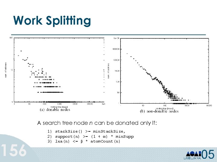Work Splitting 156 A search tree node n can be donated only if: 1) stack. Size() >= min. Stack. Size, 2) support(n) >= (1 + α) * min. Supp 3) lxa(n) <= β * atom. Count(n)

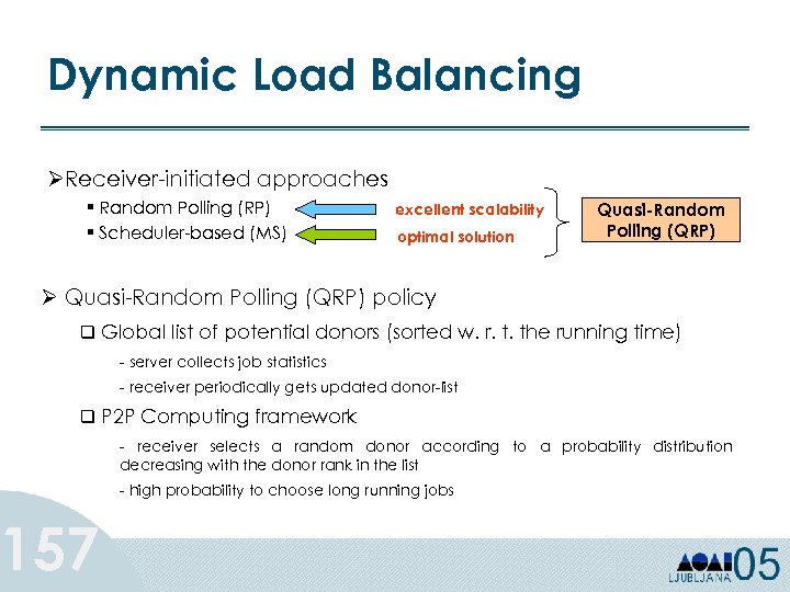Dynamic Load Balancing ØReceiver-initiated approaches § Random Polling (RP) § Scheduler-based (MS) excellent scalability optimal solution Quasi-Random Polling (QRP) Ø Quasi-Random Polling (QRP) policy q Global list of potential donors (sorted w. r. t. the running time) - server collects job statistics - receiver periodically gets updated donor-list q P 2 P Computing framework 157 - receiver selects a random donor according to a probability distribution decreasing with the donor rank in the list - high probability to choose long running jobs

Issues Ø Penalty for global synchronization § “Adaptive” application § Asynchronous communication Ø Highly irregular problem § Difficulty in predicting work loads Ø Heavy work loads may delay message processing Ø Large-scale multi-domain heterogeneous computing environment § Network latency and delay tolerant 158

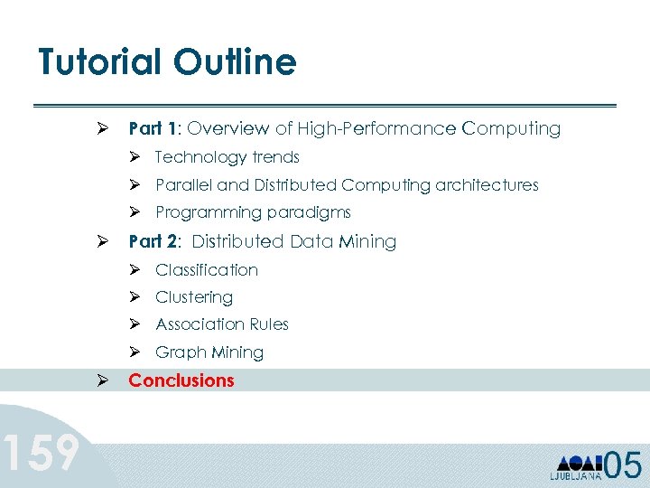Tutorial Outline 159 Ø Part 1: Overview of High-Performance Computing Ø Technology trends Ø Parallel and Distributed Computing architectures Ø Programming paradigms Ø Part 2: Distributed Data Mining Ø Classification Ø Clustering Ø Association Rules Ø Graph Mining Ø Conclusions

Large-scale Parallel KDD Systems 160 Data • Terabyte-sized datasets • Centralized or distributed datasets • Incremental changes (refine knowledge as data changes) • Heterogeneous data sources

Large-scale Parallel KDD Systems 161 Software • Pre-processing, mining, post-processing • Interactive (anytime mining) • Modular (rapid development) • Web services • Workflow management tool integration • Fault and latency tolerant • Highly scalable

Large-scale Parallel KDD Systems 162 Computing Infrastructure • Clusters already widespread • Multi-domain heterogeneous • Data and computational Grids • Dynamic resource aggregation (P 2 P) • Self-managing

Research Directions 163 • Fast algorithms: different mining tasks – Classification, clustering, associations, etc. – Incorporating concept hierarchies • Parallelism and scalability – – – Millions of records Thousands of attributes/dimensions Single pass algorithms Sampling Parallel I/O and file systems

Research Directions (contd. ) 164 • Parallel Ensemble Learning parallel execution of different data mining algorithms and techniques that can be integrated to obtain a better model. • Not just high performance but also high accuracy

Research Directions (contd. ) 165 • Tight database integration – – Push common primitives inside DBMS Use multiple tables Use efficient indexing techniques Caching strategies for sequence of data mining operations – Data mining query language and parallel query optimization

Research Directions (contd. ) 166 • Understandability: too many patterns – – Incorporate background knowledge Integrate constraints Meta-level mining Visualization, exploration • Usability: build a complete system – Pre-processing, mining, post-processing, persistent management of mined results

Conclusions • Data mining is a rapidly growing field – Fueled by enormous data collection rates, and need for intelligent analysis for business and scientific gains. • Large and high-dimensional data requires new analysis techniques and algorithms. High Performance Distributed Computing is becoming an essential component in data mining and data exploration. • Many research and commercial opportunities. 167

Resources 168 Workshops • • IEEE IPDPS Workshop on Parallel and Distributed Data Mining Hi. PC Special Session on Large-Scale Data Mining ACM SIGKDD Workshop on Distributed Data Mining IEEE IPDPS Workshop on High Performance Data Mining ACM SIGKDD Workshop on Large-Scale Parallel KDD Systems ACM SIGKDD Workshop on Distributed Data Mining, IEEE IPPS Workshop on High Performance Data Mining Life. DDM, Distributed Data Mining in Life Science Books • • • A. Freitas and S. Lavington. Mining very large databases with parallel processing. Kluwer Academic Pub. , Boston, MA, 1998. M. J. Zaki and C. -T. Ho (eds). Large-Scale Parallel Data Mining. LNAI State-ofthe-Art Survey, Volume 1759, Springer-Verlag, 2000. H. Kargupta and P. Chan (eds). Advance in Distributed and Parallel Knowledge Discovery, AAAI Press, Summer 2000.

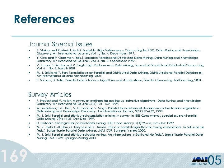References 169 Journal Special Issues • • • P. Stolorz and R. Musick (eds. ). Scalable High-Performance Computing for KDD, Data Mining and Knowledge Discovery: An International Journal, Vol. 1, No. 4, December 1997. Y. Guo and R. Grossman (eds. ). Scalable Parallel and Distributed Data Mining, Data Mining and Knowledge Discovery: An International Journal, Vol. 3, No. 3, September 1999. V. Kumar, S. Ranka and V. Singh. High Performance Data Mining, Journal of Parallel and Distributed Computing, Vol. 61, No. 3, March 2001. M. J. Zaki and Y. Pan. Special Issue on Parallel and Distributed Data Mining, Distributed and Parallel Databases: An International Journal, forthcoming, 2001. P. Srimani, D. Talia, Parallel Data Intensive Algorithms and Applications, Parallel Computing, forthcoming, 2001. Survey Articles • • • F. Provost and V. Kolluri. A survey of methods for scaling up inductive algorithms. Data Mining and Knowledge Discovery: An International Journal, 3(2): 131 --169, 1999. A. Srivastava, E. -H. Han, V. Kumar and V. Singh. Parallel formulations of decision-tree classification algorithms. Data Mining and Knowledge Discovery: An International Journal, 3(3): 237 --262, 1999. M. J. Zaki. Parallel and distributed association mining: A survey. In IEEE Concurrency special issue on Parallel Data Mining, 7(4): 14 -25, Oct-Dec 1999. D. Skillicorn. Strategies for parallel data mining. IEEE Concurrency, 7(4): 26 --35, Oct-Dec 1999. M. V. Joshi, E. -H. Han, G. Karypis and V. Kumar. Efficient parallel algorithm for mining associations. In Zaki and Ho (eds. ), Large-Scale Parallel Data Mining, LNAI 1759, Springer-Verlag 2000. M. J. Zaki. Parallel and distributed data mining: An introduction. In Zaki and Ho (eds. ), Large-Scale Parallel Data Mining, LNAI 1759, Springer-Verlag 2000.

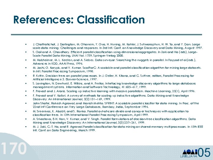References: Classification • • • 170 J. Chattratichat, J. Darlington, M. Ghanem, Y. Guo, H. Huning, M. Kohler, J. Sutiwaraphun, H. W. To, and Y. Dan. Large scale data mining: Challenges and responses. In 3 rd Intl. Conf. on Knowledge Discovery and Data Mining, August 1997. S. Goil and A. Choudhary. Efficient parallel classification using dimensional aggregates. In Zaki and Ho (eds), Large. Scale Parallel Data Mining, LNAI Vol. 1759, Springer-Verlag 2000. M. Holsheimer, M. L. Kersten, and A. Siebes. Data surveyor: Searching the nuggets in parallel. In Fayyad et al. (eds. ), Advances in KDD, AAAI Press, 1996. M. Joshi, G. Karypis, and V. Kumar. Scal. Par. C: A scalable and parallel classification algorithm for mining large datasets. In Intl. Parallel Processing Symposium, 1998. R. Kufrin. Decision trees on parallel processors. In J. Geller, H. Kitano, and C. Suttner, editors, Parallel Processing for Artificial Intelligence 3. Elsevier-Science, 1997. S. Lavington, N. Dewhurst, E. Wilkins, and A. Freitas. Interfacing knowledge discovery algorithms to large databases management systems. Information and Software Technology, 41: 605 --617, 1999. F. Provost and J. Aronis. Scaling up inductive learning with massive parallelism. Machine Learning, 23(1), April 1996. F. Provost and V. Kolluri. A survey of methods for scaling up inductive algorithms. Data Mining and Knowledge Discovery: An International Journal, 3(2): 131 --169, 1999. John Shafer, Rakesh Agrawal, and Manish Mehta. SPRINT: A scalable parallel classifier for data mining. In Proc. of the 22 nd Int'l Conference on Very Large Databases, Bombay, India, September 1996. M. Sreenivas, K. Alsabti, and S. Ranka. Parallel out-of-core divide and conquer techniques with application to classification trees. In 13 th International Parallel Processing Symposium, April 1999. A. Srivastava, E-H. Han, V. Kumar, and V. Singh. Parallel formulations of decision-tree classification algorithms. Data Mining and Knowledge Discovery: An International Journal, 3(3): 237 --261, 1999. M. J. Zaki, C. -T. Ho, and R. Agrawal. Parallel classification for data mining on shared-memory multiprocessors. In 15 th IEEE Intl. Conf. on Data Engineering, March 1999.

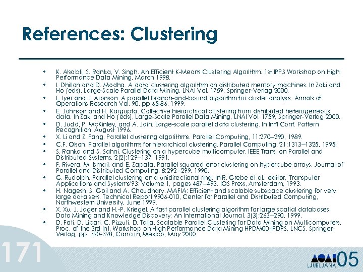References: Clustering • • • • 171 K. Alsabti, S. Ranka, V. Singh. An Efficient K-Means Clustering Algorithm. 1 st IPPS Workshop on High Performance Data Mining, March 1998. I. Dhillon and D. Modha. A data clustering algorithm on distributed memory machines. In Zaki and Ho (eds), Large-Scale Parallel Data Mining, LNAI Vol. 1759, Springer-Verlag 2000. L. Iyer and J. Aronson. A parallel branch-and-bound algorithm for cluster analysis. Annals of Operations Research Vol. 90, pp 65 -86, 1999. E. Johnson and H. Kargupta. Collective hierarchical clustering from distributed heterogeneous data. In Zaki and Ho (eds), Large-Scale Parallel Data Mining, LNAI Vol. 1759, Springer-Verlag 2000. D. Judd, P. Mc. Kinley, and A. Jain. Large-scale parallel data clustering. In Int'l Conf. Pattern Recognition, August 1996. X. Li and Z. Fang. Parallel clustering algorithms. Parallel Computing, 11: 270 --290, 1989. C. F. Olson. Parallel algorithms for hierarchical clustering. Parallel Computing, 21: 1313 --1325, 1995. S. Ranka and S. Sahni. Clustering on a hypercube multicomputer. IEEE Trans. on Parallel and Distributed Systems, 2(2): 129 --137, 1991. F. Rivera, M. Ismail, and E. Zapata. Parallel squared error clustering on hypercube arrays. Journal of Parallel and Distributed Computing, 8: 292 --299, 1990. G. Rudolph. Parallel clustering on a unidirectional ring. In R. Grebe et al. , editor, Transputer Applications and Systems'93: Volume 1, pages 487 --493. IOS Press, Amsterdam, 1993. H. Nagesh, S. Goil and A. Choudhary. MAFIA: Efficient and scalable subspace clustering for very large data sets. Technical Report 9906 -010, Center for Parallel and Distributed Computing, Northwestern University, June 1999. X. Xu, J. Jager and H. -P. Kriegel. A fast parallel clustering algorithm for large spatial databases. Data Mining and Knowledge Discovery: An International Journal. 3(3): 263 --290, 1999. D. Foti, D. Lipari, C. Pizzuti, D. Talia, Scalable Parallel Clustering for Data Mining on Multicomputers, Proc. of the 3 rd Int. Workshop on High Performance Data Mining HPDM 00 -IPDPS, LNCS, Springer. Verlag, pp. 390 -398, Cancun, Mexico, May 2000.

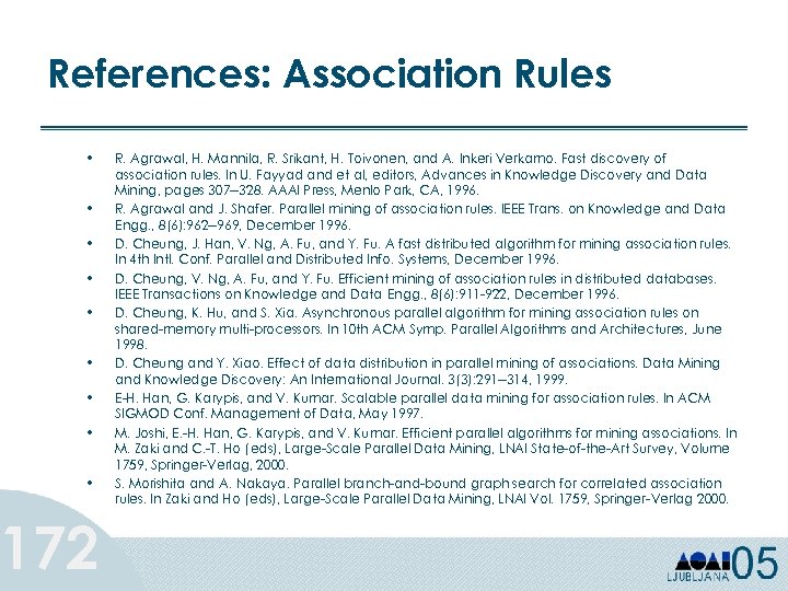References: Association Rules • • • 172 R. Agrawal, H. Mannila, R. Srikant, H. Toivonen, and A. Inkeri Verkamo. Fast discovery of association rules. In U. Fayyad and et al, editors, Advances in Knowledge Discovery and Data Mining, pages 307 --328. AAAI Press, Menlo Park, CA, 1996. R. Agrawal and J. Shafer. Parallel mining of association rules. IEEE Trans. on Knowledge and Data Engg. , 8(6): 962 --969, December 1996. D. Cheung, J. Han, V. Ng, A. Fu, and Y. Fu. A fast distributed algorithm for mining association rules. In 4 th Intl. Conf. Parallel and Distributed Info. Systems, December 1996. D. Cheung, V. Ng, A. Fu, and Y. Fu. Efficient mining of association rules in distributed databases. IEEE Transactions on Knowledge and Data Engg. , 8(6): 911 -922, December 1996. D. Cheung, K. Hu, and S. Xia. Asynchronous parallel algorithm for mining association rules on shared-memory multi-processors. In 10 th ACM Symp. Parallel Algorithms and Architectures, June 1998. D. Cheung and Y. Xiao. Effect of data distribution in parallel mining of associations. Data Mining and Knowledge Discovery: An International Journal. 3(3): 291 --314, 1999. E-H. Han, G. Karypis, and V. Kumar. Scalable parallel data mining for association rules. In ACM SIGMOD Conf. Management of Data, May 1997. M. Joshi, E. -H. Han, G. Karypis, and V. Kumar. Efficient parallel algorithms for mining associations. In M. Zaki and C. -T. Ho (eds), Large-Scale Parallel Data Mining, LNAI State-of-the-Art Survey, Volume 1759, Springer-Verlag, 2000. S. Morishita and A. Nakaya. Parallel branch-and-bound graph search for correlated association rules. In Zaki and Ho (eds), Large-Scale Parallel Data Mining, LNAI Vol. 1759, Springer-Verlag 2000.

References: Associations (contd. ) • • • 173 A. Mueller. Fast sequential and parallel algorithms for association rule mining: A comparison. Technical Report CS-TR-3515, University of Maryland, College Park, August 1995. J. S. Park, M. Chen, and P. S. Yu. Efficient parallel data mining for association rules. In ACM Intl. Conf. Information and Knowledge Management, November 1995. T. Shintani and M. Kitsuregawa. Hash based parallel algorithms for mining association rules. In 4 th Intl. Conf. Parallel and Distributed Info. Systems, December 1996. T. Shintani and M. Kitsuregawa. Parallel algorithms for mining generalized association rules with classification hierarchy. In ACM SIGMOD International Conference on Management of Data, May 1998. M. Tamura and M. Kitsuregawa. Dynamic load balancing for parallel association rule mining on heterogeneous PC cluster systems. In 25 th Int'l Conf. on Very Large Data Bases, September 1999. M. J. Zaki. Parallel and distributed association mining: A survey. IEEE Concurrency, 7(4): 14 --25, October-December 1999. M. J. Zaki, M. Ogihara, S. Parthasarathy, and W. Li. Parallel data mining for association rules on shared-memory multi-processors. In Supercomputing'96, November 1996. M. J. Zaki, S. Parthasarathy, M. Ogihara, and W. Li. New algorithms for fast discovery of association rules. In 3 rd Intl. Conf. on Knowledge Discovery and Data Mining, August 1997. M. J. Zaki, S. Parthasarathy, M. Ogihara, and W. Li. Parallel algorithms for fast discovery of association rules. Data Mining and Knowledge Discovery: An International Journal, 1(4): 343 -373, December 1997. M. J. Zaki, S. Parthasarathy, W. Li, A Localized Algorithm for Parallel Association Mining, 9 th Annual ACM Symposium on Parallel Algorithms and Architectures (SPAA), June, 1997.

References: Subgraph Mining • • • 174 G. Di Fatta and M. R. Berthold. Distributed Mining of Molecular Fragments. IEEE DM-Grid Workshop of the Int. Conf. on Data Mining (ICDM 2004, Brighton, UK), November 1 -4, 2004. M. Desphande and M. Kuramochi and G. Karypis. Automated Approaches for Classifying Structures. Proc. of Workshop on Data Mining in Bioinformatics (Bio. KDD), 2002, pp. 11 -18. X. Yan and J. Han. g. Span: Graph-Based Substructure Pattern Mining. Proceedings of the IEEE International Conference on Data Mining ICDM, Maebashi City, Japan, 2002. S. Kramer and L. de Raedt and C. Helma. Molecular Feature Mining in HIV Data. Proc. of 7 th Int. Conf. on Knowledge Discovery and Data Mining, (KDD-2001, San Francisco, CA, 2001, pp. 136 -143. Takashi Washio and Hiroshi Motoda. State of the art of graph-based data mining. ACM SIGKDD Explorations Newsletter, July 2003 Vol. 5, pp. 59 -68. Chao Wang and Srinivasan Parthasarathy. Parallel Algorithms for Mining Frequent Structural Motifs in Scientific Data. ICS’ 04, June 26–July 1, 2004, Saint-Malo, France.