AAMP Training Materials Module 2 2 Modeling Smallholder

AAMP Training Materials Module 2. 2: Modeling Smallholder Commercialization Nicholas Minot (IFPRI) n. minot@ifpri. org

Contents • Agricultural commercialization conceptual framework • Agricultural household models before and after 1985 – Separable vs Non-Separable household models • Household modeling exercises • Conclusions • Resources

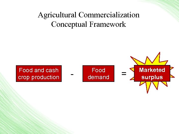Agricultural Commercialization Conceptual Framework Food and cash crop production - Food demand = Marketed surplus

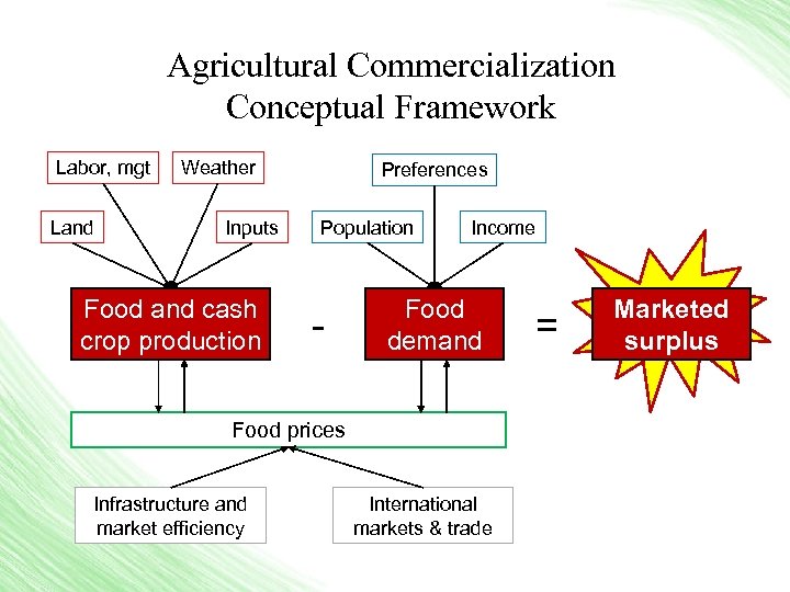Agricultural Commercialization Conceptual Framework Labor, mgt Land Weather Inputs Food and cash crop production Preferences Population - Income Food demand Food prices Infrastructure and market efficiency International markets & trade = Marketed surplus

Agricultural household models – Before 1985 • “Separable household models” – Maximize household income – Allocate income among consumption goods to maximize utility • “Separable” in that production decisions are not affected by consumption decisions • Marketed surplus is difference between optimal quantity of production and optimal quantity of consumption – They could only be equal by coincidence so this should only occur rarely

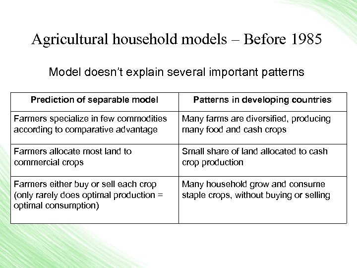Agricultural household models – Before 1985 Model doesn’t explain several important patterns Prediction of separable model Patterns in developing countries Farmers specialize in few commodities according to comparative advantage Many farms are diversified, producing many food and cash crops Farmers allocate most land to commercial crops Small share of land allocated to cash crop production Farmers either buy or sell each crop (only rarely does optimal production = optimal consumption) Many household grow and consume staple crops, without buying or selling

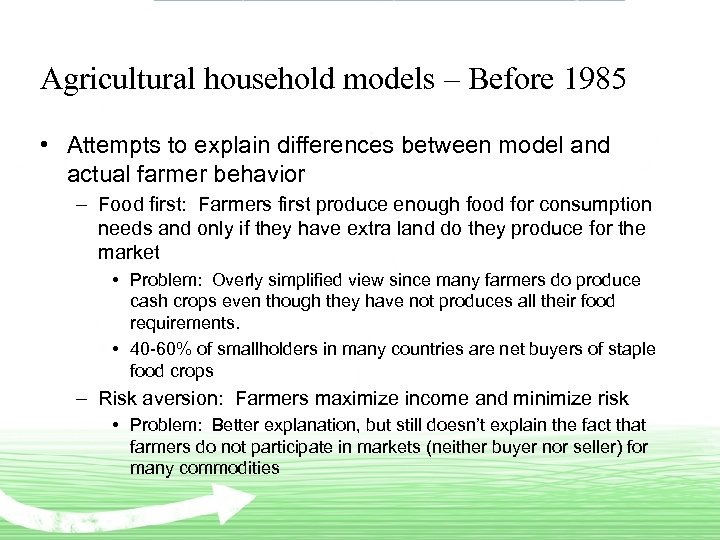Agricultural household models – Before 1985 • Attempts to explain differences between model and actual farmer behavior – Food first: Farmers first produce enough food for consumption needs and only if they have extra land do they produce for the market • Problem: Overly simplified view since many farmers do produce cash crops even though they have not produces all their food requirements. • 40 -60% of smallholders in many countries are net buyers of staple food crops – Risk aversion: Farmers maximize income and minimize risk • Problem: Better explanation, but still doesn’t explain the fact that farmers do not participate in markets (neither buyer nor seller) for many commodities

Agricultural household models – After 1985 • Non-separable household models – Singh, Squire, & Strauss (1986) Agricultural Household Models – Models incorporating transaction costs, ie cost of buying or selling a commodity – Creates a gap between a) price household can buy at and b) price it can sell at – Example: • Suppose market price of maize is 300, but it costs 50 to transport it to the market or to transport from market to household • Farmer can pay 350 to purchase maize or he can earn 250 from selling maize • If maize is worth 290 to household, it is not worth buying or selling maize, so household does not participate in market

Agricultural household models – After 1985 • Why do transaction costs make models non-separable? – Cannot calculate profit-maximizing production without knowing consumption preferences – Consumption preferences whether household is buyer or seller price of commodity for household profit maximization – Thus, consumption preferences and profit maximizing income must be solve simultaneously • Spatial arbitrage between household & market – Shadow price (Ph) for household • • Ph = Pm +t if household is buying commodity Ph = Pm – t if household is selling commodity Pm+t > Ph > Pm-t if household neither sells nor buys The larger is t, the more likely household neither sells nor buys

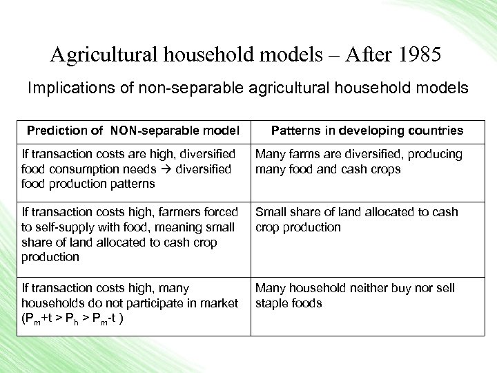Agricultural household models – After 1985 Implications of non-separable agricultural household models Prediction of NON-separable model Patterns in developing countries If transaction costs are high, diversified food consumption needs diversified food production patterns Many farms are diversified, producing many food and cash crops If transaction costs high, farmers forced to self-supply with food, meaning small share of land allocated to cash crop production Small share of land allocated to cash crop production If transaction costs high, many households do not participate in market (Pm+t > Ph > Pm-t ) Many household neither buy nor sell staple foods

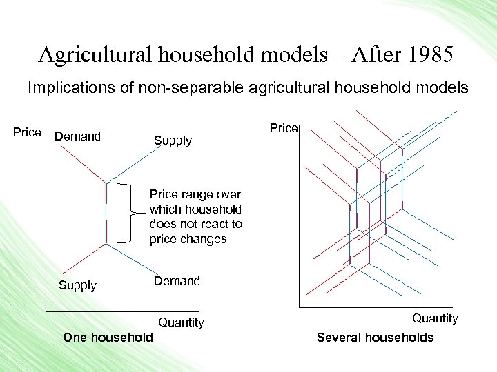Agricultural household models – After 1985 Implications of non-separable agricultural household models Price Demand Supply Price range over which household does not react to price changes Supply Demand Quantity One household Quantity Several households

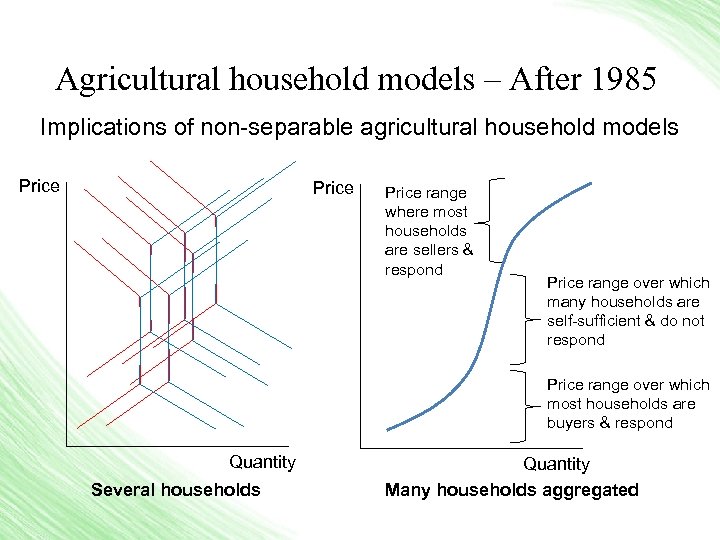Agricultural household models – After 1985 Implications of non-separable agricultural household models Price range where most households are sellers & respond Price range over which many households are self-sufficient & do not respond Price range over which most households are buyers & respond Quantity Several households Quantity Many households aggregated

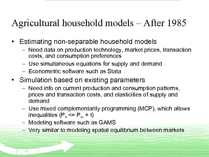Agricultural household models – After 1985 • Estimating non-separable household models – Need data on production technology, market prices, transaction costs, and consumption preferences – Use simultaneous equations for supply and demand – Econometric software such as Stata • Simulation based on existing parameters – Need info on current production and consumption patterns, prices and transaction costs, and elasticities of supply and demand – Use mixed complementarity programming (MCP), which allows inequalities (Ph <= Pm + t) – Modeling software such as GAMS – Very similar to modeling spatial equilibrium between markets

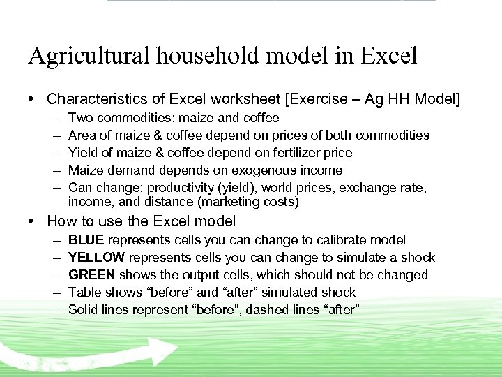Agricultural household model in Excel • Characteristics of Excel worksheet [Exercise – Ag HH Model] – – – Two commodities: maize and coffee Area of maize & coffee depend on prices of both commodities Yield of maize & coffee depend on fertilizer price Maize demand depends on exogenous income Can change: productivity (yield), world prices, exchange rate, income, and distance (marketing costs) • How to use the Excel model – – – BLUE represents cells you can change to calibrate model YELLOW represents cells you can change to simulate a shock GREEN shows the output cells, which should not be changed Table shows “before” and “after” simulated shock Solid lines represent “before”, dashed lines “after”

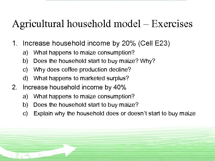Agricultural household model – Exercises 1. Increase household income by 20% (Cell E 23) a) b) c) d) What happens to maize consumption? Does the household start to buy maize? Why does coffee production decline? What happens to marketed surplus? 2. Increase household income by 40% a) What happens to maize consumption? b) Does the household start to buy maize? c) Explain why the household does or doesn’t start to buy maize

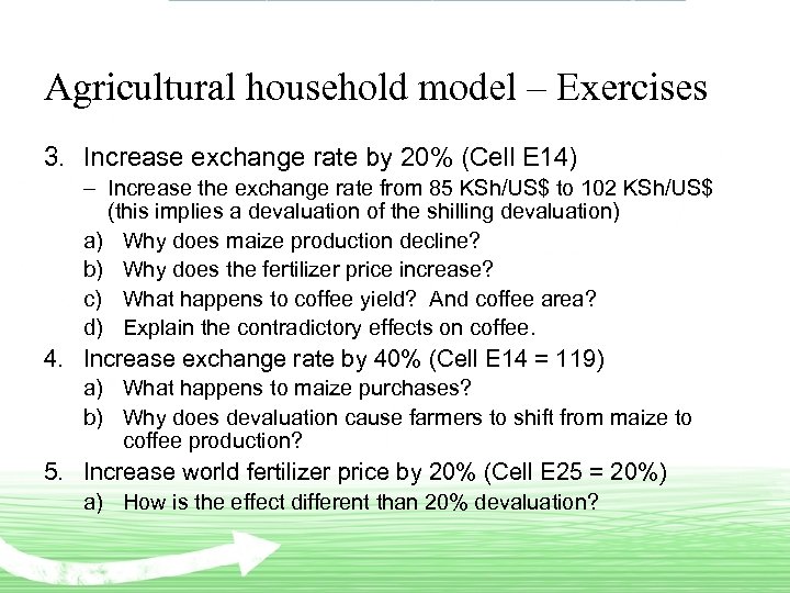Agricultural household model – Exercises 3. Increase exchange rate by 20% (Cell E 14) – Increase the exchange rate from 85 KSh/US$ to 102 KSh/US$ (this implies a devaluation of the shilling devaluation) a) Why does maize production decline? b) Why does the fertilizer price increase? c) What happens to coffee yield? And coffee area? d) Explain the contradictory effects on coffee. 4. Increase exchange rate by 40% (Cell E 14 = 119) a) What happens to maize purchases? b) Why does devaluation cause farmers to shift from maize to coffee production? 5. Increase world fertilizer price by 20% (Cell E 25 = 20%) a) How is the effect different than 20% devaluation?

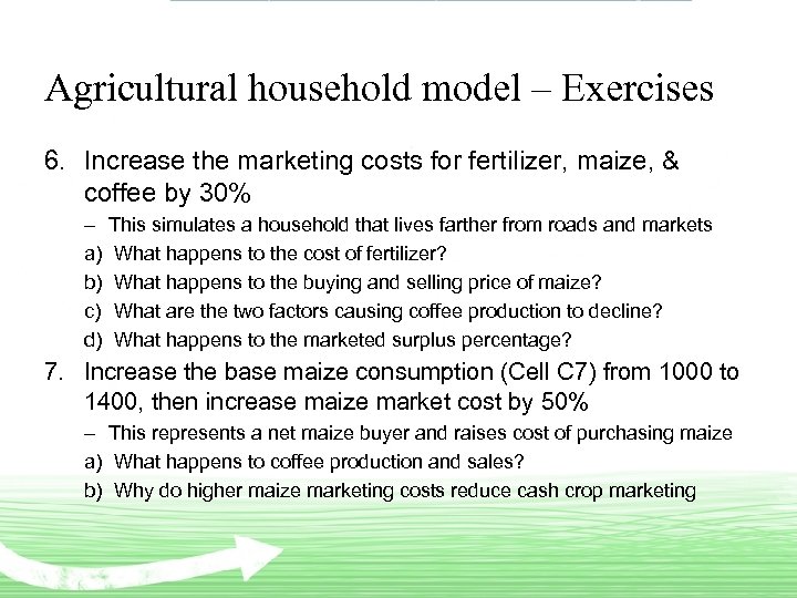Agricultural household model – Exercises 6. Increase the marketing costs for fertilizer, maize, & coffee by 30% – a) b) c) d) This simulates a household that lives farther from roads and markets What happens to the cost of fertilizer? What happens to the buying and selling price of maize? What are the two factors causing coffee production to decline? What happens to the marketed surplus percentage? 7. Increase the base maize consumption (Cell C 7) from 1000 to 1400, then increase maize market cost by 50% – This represents a net maize buyer and raises cost of purchasing maize a) What happens to coffee production and sales? b) Why do higher maize marketing costs reduce cash crop marketing

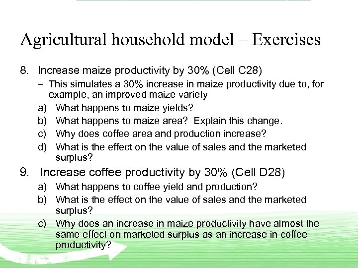Agricultural household model – Exercises 8. Increase maize productivity by 30% (Cell C 28) – This simulates a 30% increase in maize productivity due to, for example, an improved maize variety a) What happens to maize yields? b) What happens to maize area? Explain this change. c) Why does coffee area and production increase? d) What is the effect on the value of sales and the marketed surplus? 9. Increase coffee productivity by 30% (Cell D 28) a) What happens to coffee yield and production? b) What is the effect on the value of sales and the marketed surplus? c) Why does an increase in maize productivity have almost the same effect on marketed surplus as an increase in coffee productivity?

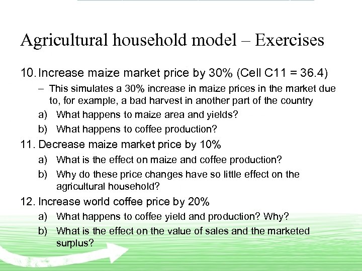Agricultural household model – Exercises 10. Increase maize market price by 30% (Cell C 11 = 36. 4) – This simulates a 30% increase in maize prices in the market due to, for example, a bad harvest in another part of the country a) What happens to maize area and yields? b) What happens to coffee production? 11. Decrease maize market price by 10% a) What is the effect on maize and coffee production? b) Why do these price changes have so little effect on the agricultural household? 12. Increase world coffee price by 20% a) What happens to coffee yield and production? Why? b) What is the effect on the value of sales and the marketed surplus?

Conclusions • Rising income dampens commercialization if household is self-sufficient • Devaluation (or depreciation) increases commercialization by shifting incentives toward export crops • Distance to market and high marketing costs reduce commercialization by reducing fertilizer use & yields and lowering farm gate price of commercial crops • More…

Conclusions • If household is net buyer of food, high marketing costs reduce commercialization by diverting land from commercial crops to food crops • Higher productivity in staple food crop contributes to commercialization by making land available • Higher maize prices have no effect on self-sufficient households, which explains inelasticity of supply of staple foods

Resources • Singh, I. , L. Squire, & J. Strauss. 1986. Agricultural household models: Extension, application and policy. Baltimore: Johns Hopkins University Press. • de Janvry, A. , M. Fafchamps , and E. Sadoulet. 1991. Peasant household behavior with missing markets: some paradoxes explained. Economic Journal 101 (409): 1400 -17, November. • Taylor, J. 2003. Agricultural Household Models: Genesis, Evolution, and Extensions. Review of Economics of the Household, Vol. 1, No. 1. http: //www. reap. ucdavis. edu/research/Agricultural. pdf • Renkow, M. Agricultural household models. Lecture notes. http: //www. agecon. ncsu. edu/faculty/renkow/ECG_540/05_household. pdf