914e5a3ea335518ce353a09874a80f71.ppt
- Количество слайдов: 26
A SIMPLE INTRODUCTION TO DYNAMIC PROGRAMMING
PROBLEM SET-UP Problem is arrayed as a set of decisions made over time. System has a discrete state Each decision results in some reward or cost, and results in the system being moved to another state. Usually has a finite number of transitions. Transitions can be probabilistic, as can the rewards. Solution is a decision strategy that maximizes summed reward (minimizes cost)
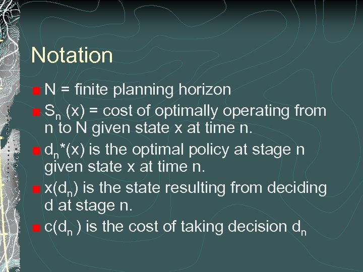
Notation N = finite planning horizon Sn (x) = cost of optimally operating from n to N given state x at time n. dn*(x) is the optimal policy at stage n given state x at time n. x(dn) is the state resulting from deciding d at stage n. c(dn ) is the cost of taking decision dn
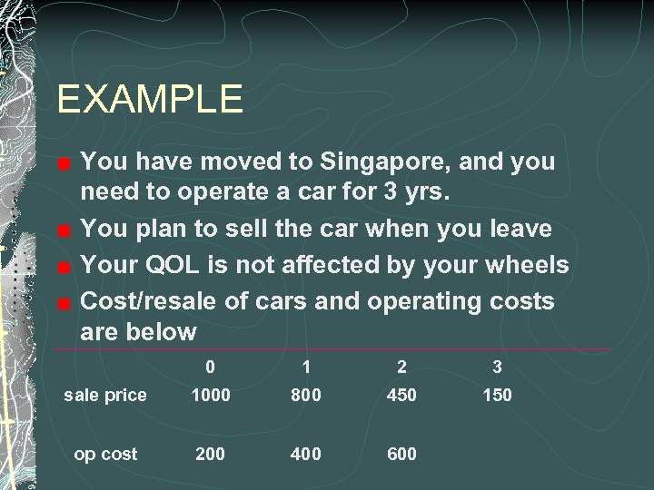
EXAMPLE You have moved to Singapore, and you need to operate a car for 3 yrs. You plan to sell the car when you leave Your QOL is not affected by your wheels Cost/resale of cars and operating costs are below 0 1 2 3 sale price 1000 800 450 150 op cost 200 400 600
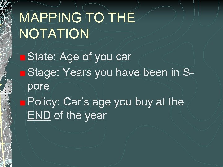
MAPPING TO THE NOTATION State: Age of you car Stage: Years you have been in Spore Policy: Car’s age you buy at the END of the year
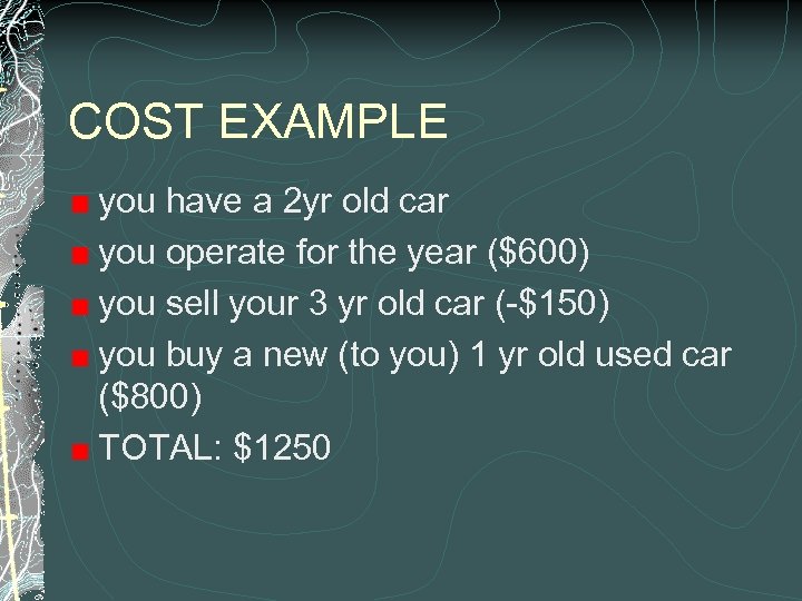
COST EXAMPLE you have a 2 yr old car you operate for the year ($600) you sell your 3 yr old car (-$150) you buy a new (to you) 1 yr old used car ($800) TOTAL: $1250
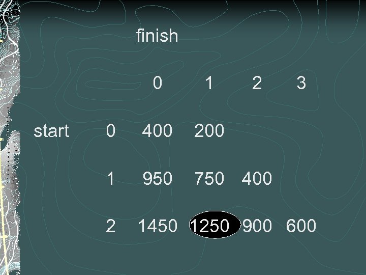
finish 0 start 1 2 3 0 400 200 1 950 750 400 2 1450 1250 900 600
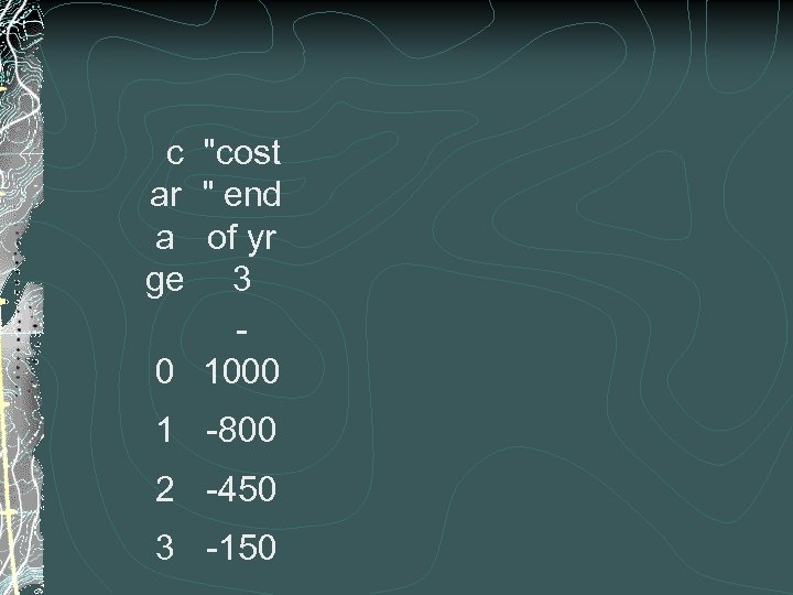
c "cost ar " end a of yr ge 3 0 1000 1 -800 2 -450 3 -150
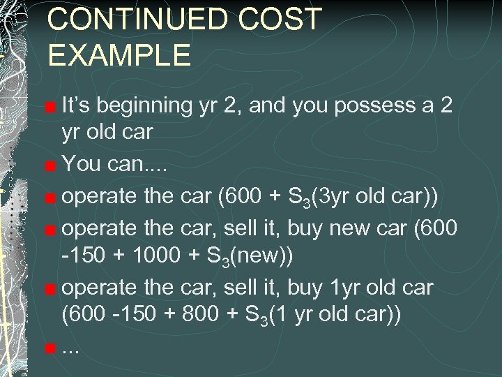
CONTINUED COST EXAMPLE It’s beginning yr 2, and you possess a 2 yr old car You can. . operate the car (600 + S 3(3 yr old car)) operate the car, sell it, buy new car (600 -150 + 1000 + S 3(new)) operate the car, sell it, buy 1 yr old car (600 -150 + 800 + S 3(1 yr old car)). . .
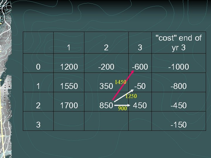
1 2 3 "cost" end of yr 3 0 1200 -600 -1000 -50 -800 1 1550 350 1450 1250 2 1700 850 3 900 450 -150
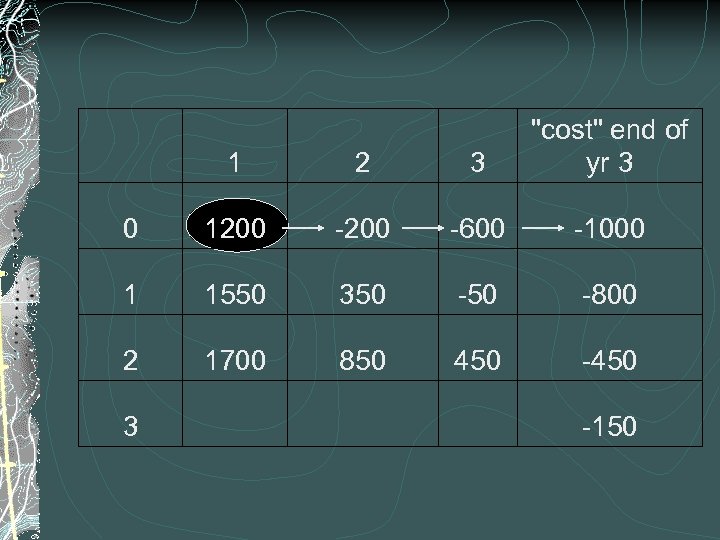
1 2 3 "cost" end of yr 3 0 1200 -600 -1000 1 1550 350 -800 2 1700 850 450 -450 3 -150
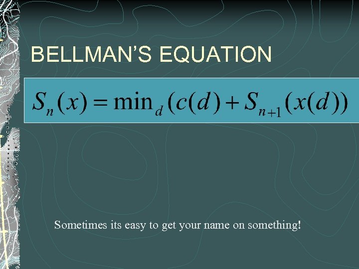
BELLMAN’S EQUATION Sometimes its easy to get your name on something!
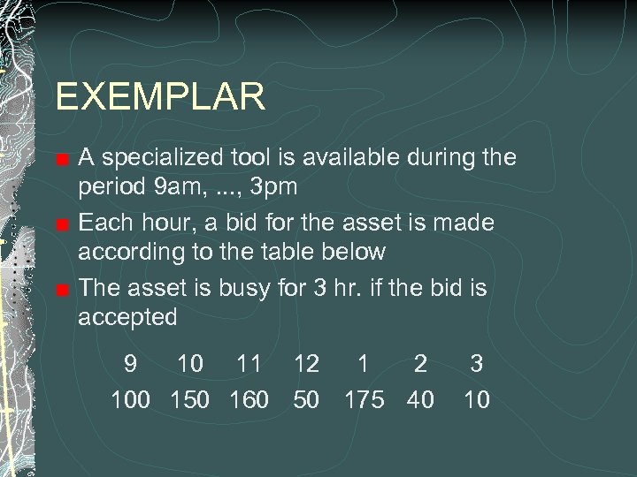
EXEMPLAR A specialized tool is available during the period 9 am, . . . , 3 pm Each hour, a bid for the asset is made according to the table below The asset is busy for 3 hr. if the bid is accepted 9 10 11 12 1 2 100 150 160 50 175 40 3 10
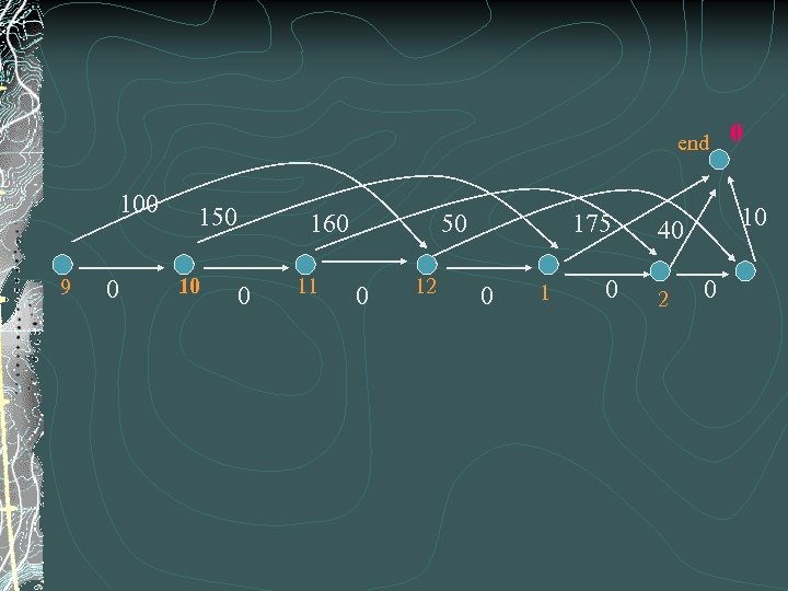
end 100 9 0 150 10 160 0 11 50 0 12 175 0 10 40 2 0 0
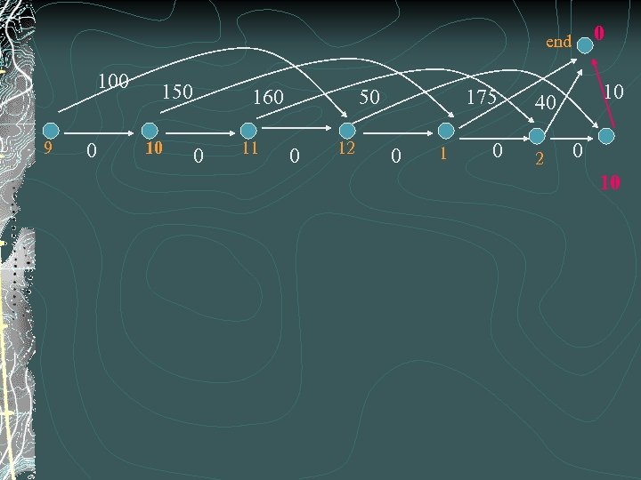
0 end 100 9 0 150 10 160 0 11 50 0 12 175 0 10 40 2 0 10
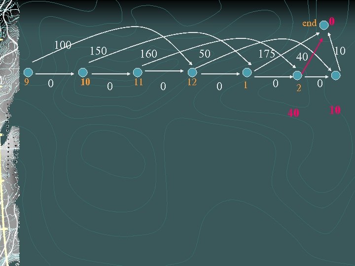
0 end 100 9 0 150 10 160 0 11 50 0 12 175 0 10 40 2 40 0 10
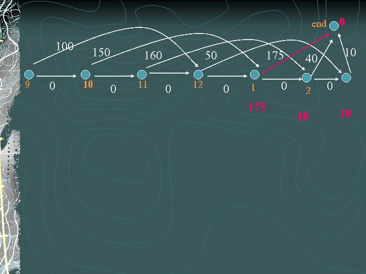
0 end 100 9 0 150 10 160 0 11 50 0 12 175 0 10 40 2 40 0 10
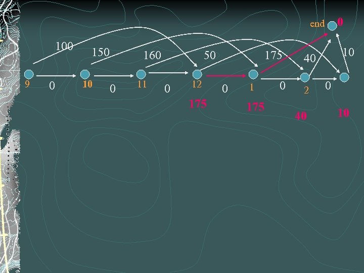
0 end 100 9 0 150 10 160 0 11 50 0 12 175 0 10 40 2 40 0 10
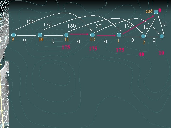
0 end 100 9 0 150 10 160 0 11 175 50 0 12 175 0 10 40 2 40 0 10
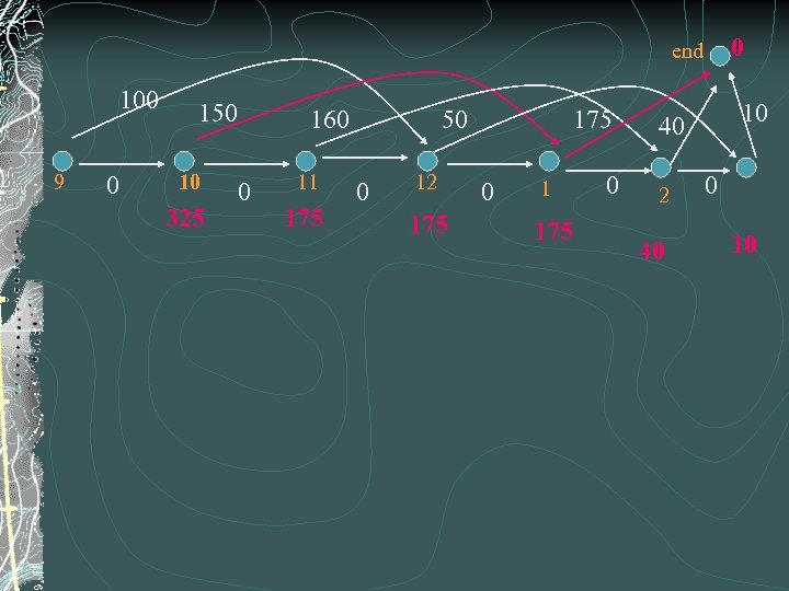
0 end 100 9 0 150 10 325 160 0 11 175 50 0 12 175 0 10 40 2 40 0 10
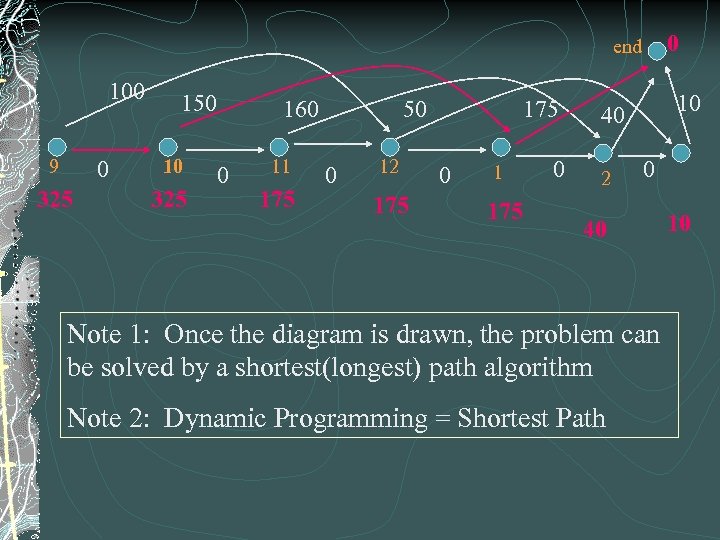
0 end 100 9 0 325 150 10 325 160 0 11 175 50 0 12 175 0 10 40 2 0 40 Note 1: Once the diagram is drawn, the problem can be solved by a shortest(longest) path algorithm Note 2: Dynamic Programming = Shortest Path 10
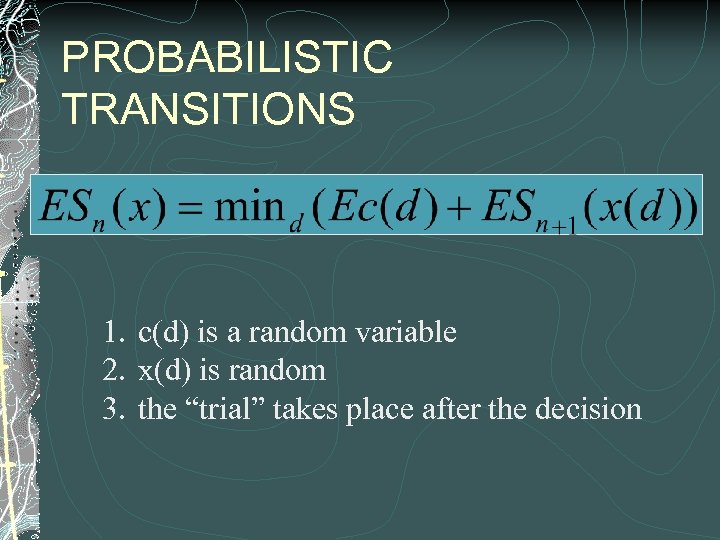
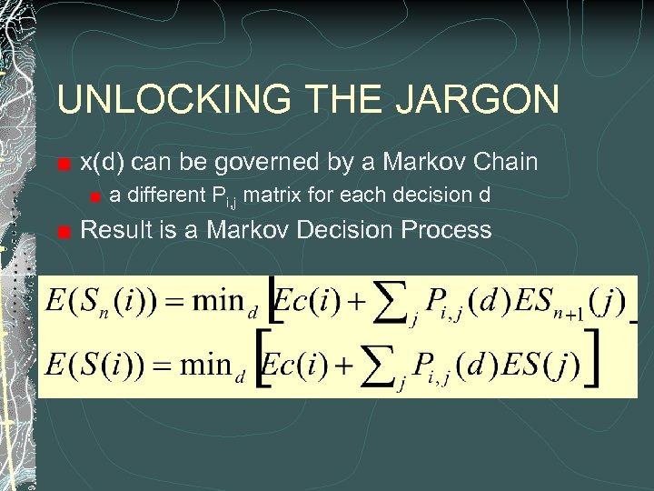
PROBABILISTIC TRANSITIONS 1. c(d) is a random variable 2. x(d) is random 3. the “trial” takes place after the decision
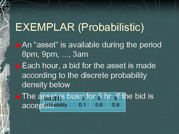
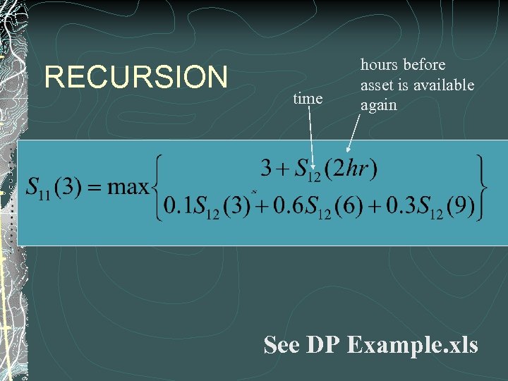
EXEMPLAR (Probabilistic) An “asset” is available during the period 8 pm, 9 pm, . . . , 3 am Each hour, a bid for the asset is made according to the discrete probability density below The asset is busy for 3 hr. if the bid is accepted
MANY APPROACHES TO FORMULATION N = 4 am Sn (x) = profit of optimally operating from n to N given state x at time n. dn*(x) is the optimal policy at stage n given state x at time n (ACCEPT, REJECT) c(dn ) is the profit of taking decision dn x(dn) is the proposed bid (3, 6, 9) or the number of hours left in the remaining engagement (1 hr, 2 hr)
RECURSION time hours before asset is available again See DP Example. xls
UNLOCKING THE JARGON x(d) can be governed by a Markov Chain a different Pi, j matrix for each decision d Result is a Markov Decision Process
914e5a3ea335518ce353a09874a80f71.ppt