A Simple -But-Powerful Test for Long-Run Event Studies

A Simple -But-Powerful Test for Long-Run Event Studies Gitit Gur-Gershgoren Eric Hughson Jaime F. Zender

Long Run Event Studies n Examine equity price behavior for extended periods (commonly 1 – 5 years) following significant corporate events q n e. g. , IPOs, SEOs, stock repurchases, stock splits, bond rating changes, mergers… Two issues are debated in the literature: - How to measure long-run abnormal performance? How to test for the significance of that performance?

Abnormal Performance BHARs measure investor experience. q But the use of BHARs can be problematic… q Long-run CARs on the other hand: q q § q CARs do not measure long-run investor experience. CARs are biased predictors of BHARs. CARs suffer from some of the same issues as BHARs, perhaps less so. However: n q q The use of CARs is statistically less problematic, and standard tests can be used. Also, most of what we know about expected returns comes from studies of monthly returns.

Inference Using BHARs Reference portfolio: q Commonly a size and book-to-market matched portfolio. n q q Pro: high power Cons: new listing bias, rebalancing bias, and skewness bias (Barber and Lyon, 1997) Skewness bias with standard (t) tests: q If the long-run BHAR is skewed enough, the test statistic is affected by a few extreme observations in the right tail of the distribution. n q Over-rejection in samples where the big returns don’t occur.

Inference Using BHARs Control Firm Approach q Pros: n q q § § Lack of biases. Well-specified test. i. e. , a 5% test rejects 5% of the time under the null. Annual BHAR skewness is 0. 4 instead of 8. 0. Con: low power n q q q BHAR = rsample firm – rcontrol firm Var(BHAR) = var(rsample firm) + var(rcontrol firm) – 2 cov(●) Even with good matching, that covariance term isn’t big. BL (1997) best effort: n q Match on size and then book-to-market.

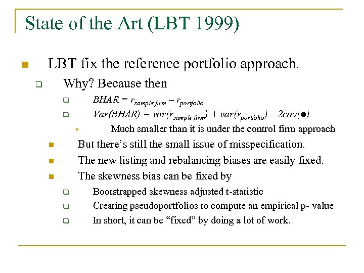
State of the Art (LBT 1999) LBT fix the reference portfolio approach. n Why? Because then q q q § BHAR = rsample firm – rportfolio Var(BHAR) = var(rsample firm) + var(rportfolio) – 2 cov(●) Much smaller than it is under the control firm approach But there’s still the small issue of misspecification. The new listing and rebalancing biases are easily fixed. The skewness bias can be fixed by n n n q q q Bootstrapped skewness adjusted t-statistic Creating pseudoportfolios to compute an empirical p- value In short, it can be “fixed” by doing a lot of work.

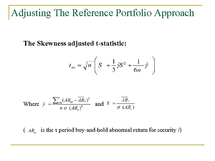
Adjusting The Reference Portfolio Approach The Skewness adjusted t-statistic: Where ( and is the τ period buy-and-hold abnormal return for security i)

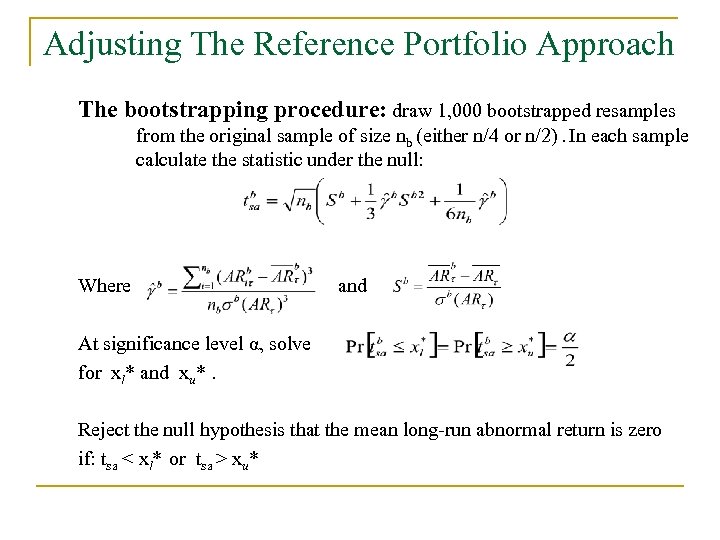
Adjusting The Reference Portfolio Approach The bootstrapping procedure: draw 1, 000 bootstrapped resamples from the original sample of size nb (either n/4 or n/2). In each sample calculate the statistic under the null: Where and At significance level α, solve for xl* and xu*. Reject the null hypothesis that the mean long-run abnormal return is zero if: tsa < xl* or tsa > xu*

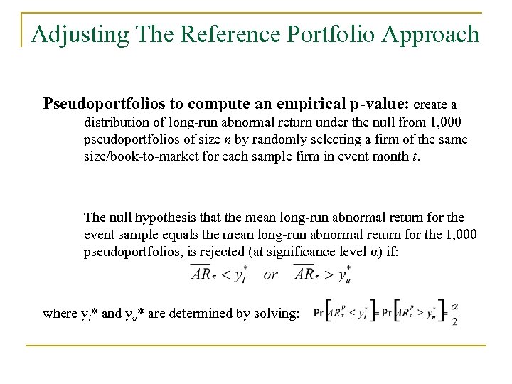
Adjusting The Reference Portfolio Approach Pseudoportfolios to compute an empirical p-value: create a distribution of long-run abnormal return under the null from 1, 000 pseudoportfolios of size n by randomly selecting a firm of the same size/book-to-market for each sample firm in event month t. The null hypothesis that the mean long-run abnormal return for the event sample equals the mean long-run abnormal return for the 1, 000 pseudoportfolios, is rejected (at significance level α) if: where yl* and yu* are determined by solving:

The Problems That Remain Nonrandom samples n q In nonrandom samples, neither of these approaches will generally yield a well-specified test (LBT). Time clustering n q Bootstrapping techniques assume independence of observations within a time period (Mitchell and Stafford (2000)). Asymmetric power n q The empirical distribution is not symmetric, therefore, power will be higher against some alternatives than others.

Our Approach n n We use the control firm approach, with multiple control firms per sample firm to increase the power of the test. This creates multiple correlated observations per event firm so we use a Wald statistic to control for the induced correlation. q The resulting test is: n n Easy to implement. Has higher power than extant tests. Is (can be) well specified in non-random samples. Is well specified when there is time clustering

Two Matching Procedures Rationale: n A very important aspect of our approach is the selection of control firms. Find a set of control firm returns that provides the greatest explanatory power for the sample firm return in the event window. Statistical (maximal R 2): n For each sample firm, we choose from a set of K potential control firms, the M that maximize the R 2 of the regression of sample firm return over all potential sets of M control firm returns that can be formed from the K candidates. q The K firms are chosen to have characteristics that explain the crosssection of average returns: size, book-to-market, beta, etc. Purely characteristic-driven: n Match solely on firm characteristics.

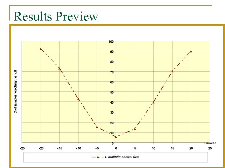
Results Preview

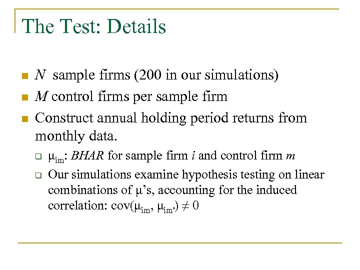
The Test: Details n n n N sample firms (200 in our simulations) M control firms per sample firm Construct annual holding period returns from monthly data. q q μim: BHAR for sample firm i and control firm m Our simulations examine hypothesis testing on linear combinations of μ’s, accounting for the induced correlation: cov(μim, μim') ≠ 0

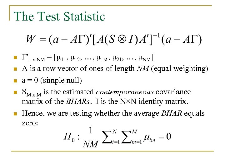
The Test Statistic n n n Γ′ 1 x NM = [μ 11, μ 12, …, μ 1 M, μ 21, …, μNM] A is a row vector of ones of length NM (equal weighting) a = 0 (simple null) SM x M is the estimated contemporaneous covariance matrix of the BHARs. I is the N×N identity matrix. Hence, we are testing whether the average BHAR equals zero:

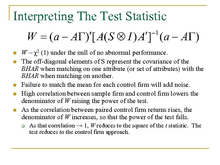
Interpreting The Test Statistic n n n W ~ χ2 (1) under the null of no abnormal performance. The off-diagonal elements of S represent the covariance of the BHAR when matching on one attribute (or set of attributes) with the BHAR when matching on another. Failure to match the mean for each control firm will add noise. High correlation between sample firm and control firm lowers the denominator of W raising the power of the test. As the correlation between paired control firm returns rises, the denominator of W increases, so that the power of the test falls. q As that correlation → 1, W reduces to the square of the t statistic. The test reduces to the control firm approach.

Control Firm Selection n Find a set of control firms whose returns provide the greatest explanatory power for the return of each sample firm in the event window, with the least noise. q q Intuitively, maximize the correlation between sample firm and control firm returns and minimize correlation of control firm returns with each other. With real stock returns: complications n Average returns on stocks vary q n You have to get the “buy and hold normal return” right. How big should M be?

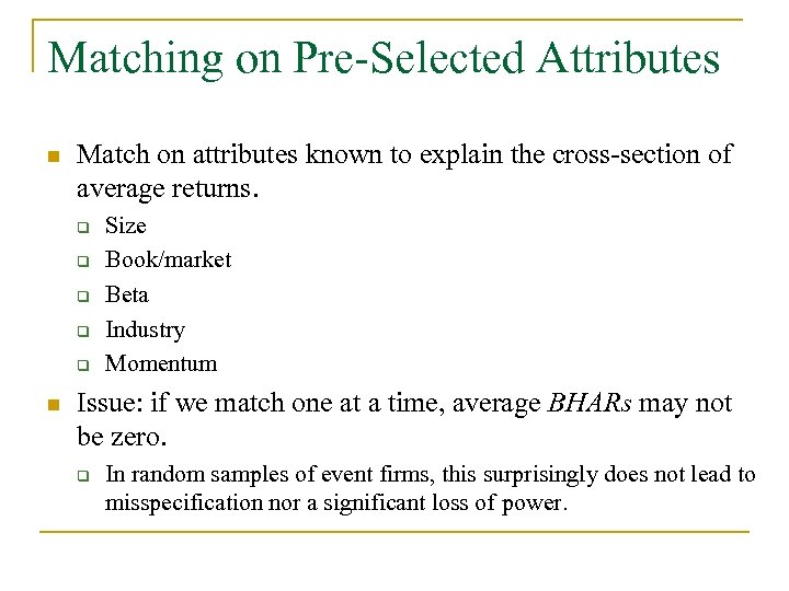
Matching on Pre-Selected Attributes n Match on attributes known to explain the cross-section of average returns. q q q n Size Book/market Beta Industry Momentum Issue: if we match one at a time, average BHARs may not be zero. q In random samples of event firms, this surprisingly does not lead to misspecification nor a significant loss of power.

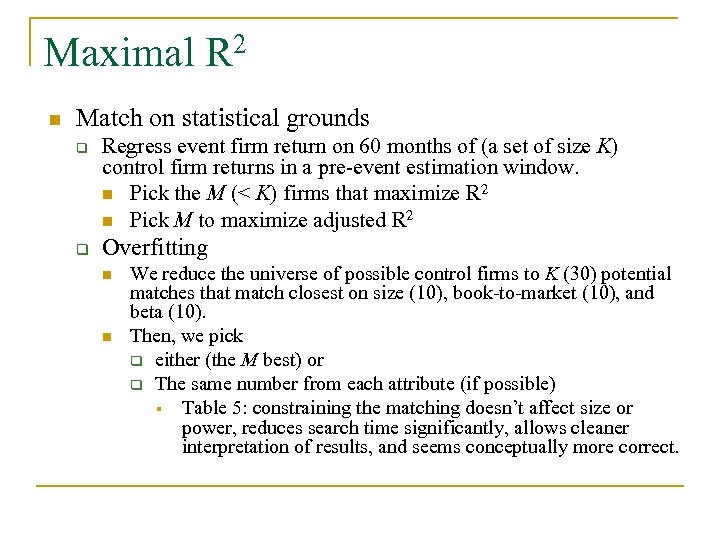
Maximal R 2 n Match on statistical grounds q q Regress event firm return on 60 months of (a set of size K) control firm returns in a pre-event estimation window. n Pick the M (< K) firms that maximize R 2 n Pick M to maximize adjusted R 2 Overfitting n n We reduce the universe of possible control firms to K (30) potential matches that match closest on size (10), book-to-market (10), and beta (10). Then, we pick q either (the M best) or q The same number from each attribute (if possible) § Table 5: constraining the matching doesn’t affect size or power, reduces search time significantly, allows cleaner interpretation of results, and seems conceptually more correct.

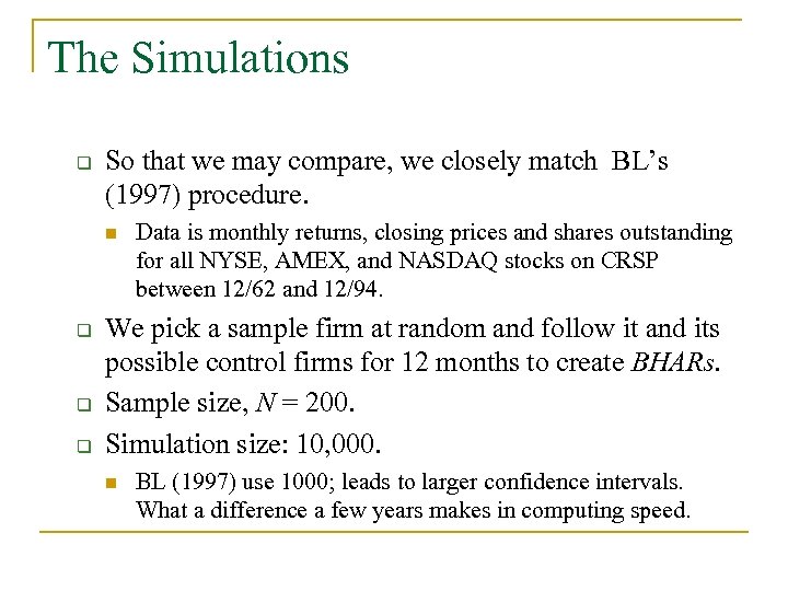
The Simulations q So that we may compare, we closely match BL’s (1997) procedure. n q q q Data is monthly returns, closing prices and shares outstanding for all NYSE, AMEX, and NASDAQ stocks on CRSP between 12/62 and 12/94. We pick a sample firm at random and follow it and its possible control firms for 12 months to create BHARs. Sample size, N = 200. Simulation size: 10, 000. n BL (1997) use 1000; leads to larger confidence intervals. What a difference a few years makes in computing speed.

How did we do ?

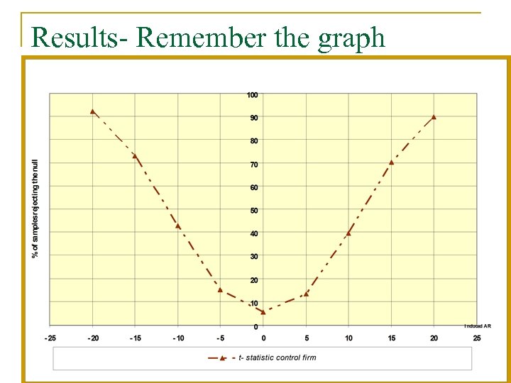
Results- Remember the graph

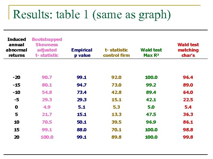
Results: table 1 (same as graph) Induced Bootstrapped annual Skewness abnormal adjusted returns t- statistic Empirical p value t- statistic control firm Wald test Max R 2 Wald test matching char’s -20 90. 7 99. 1 92. 0 100. 0 96. 4 -15 80. 1 94. 7 73. 0 99. 2 89. 0 -10 54. 8 73. 4 42. 8 89. 4 64. 0 -5 29. 3 15. 1 42. 1 22. 5 0 4. 9 5. 1 5. 3 5. 0 5. 4 5 21. 7 15. 1 13. 3 47. 5 36. 3 10 70. 5 50. 1 39. 5 96. 9 86. 1 15 99. 1 88. 0 70. 1 100. 0 98. 8 20 100. 0 99. 1 89. 8 100. 0 99. 8

Characteristic-Based Matching Does how we match matter? n Surprisingly, as long as you match the expected return, most approaches do well. q What follow are n 1. – 2. Some typical results Note how well matching by size, bookto-market and beta works. What happens if we match on size decile and then book-to-market within that decile.

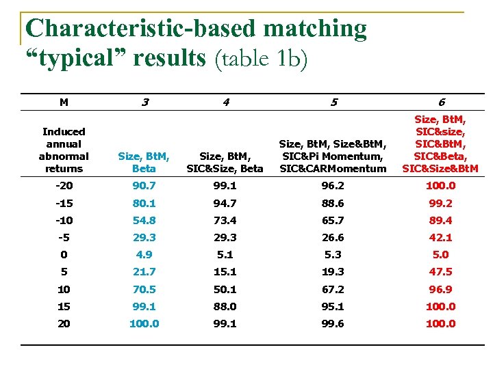
Characteristic-based matching “typical” results (table 1 b) 3 M 4 5 6 Size, Bt. M, SIC&size, SIC&Bt. M, SIC&Beta, SIC&Size&Bt. M Induced annual abnormal returns Size, Bt. M, Beta Size, Bt. M, SIC&Size, Beta Size, Bt. M, Size&Bt. M, SIC&Pi Momentum, SIC&CARMomentum -20 90. 7 99. 1 96. 2 100. 0 -15 80. 1 94. 7 88. 6 99. 2 -10 54. 8 73. 4 65. 7 89. 4 -5 29. 3 26. 6 42. 1 0 4. 9 5. 1 5. 3 5. 0 5 21. 7 15. 1 19. 3 47. 5 10 70. 5 50. 1 67. 2 96. 9 15 99. 1 88. 0 95. 1 100. 0 20 100. 0 99. 1 99. 6 100. 0

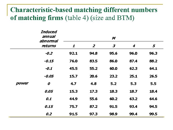
Characteristic-based matching different numbers of matching firms (table 4) (size and BTM) Induced annual abnormal returns 2 3 4 5 -0. 2 92. 1 94. 8 95. 6 96. 0 96. 3 -0. 15 76. 0 83. 5 86. 0 87. 4 88. 2 -0. 1 45. 5 55. 2 60. 0 62. 3 64. 1 -0. 05 power 1 15. 7 20. 6 23. 2 25. 1 26. 5 0 4. 7 4. 8 5. 2 5. 3 5. 5 0. 05 15. 3 17. 3 18. 7 18. 4 0. 1 44. 9 55. 6 60. 2 63. 2 64. 6 0. 15 75. 7 87. 2 91. 5 93. 4 94. 5 0. 2 91. 5 97. 3 98. 9 99. 4 99. 5 M

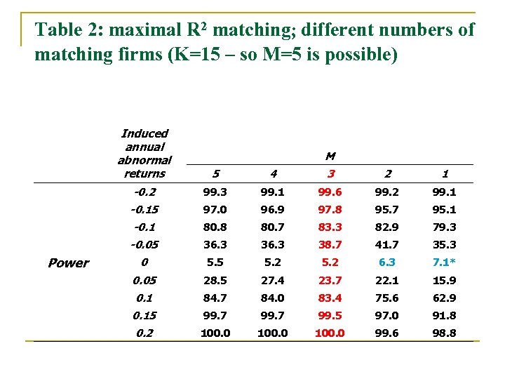
Table 2: maximal R 2 matching; different numbers of matching firms (K=15 – so M=5 is possible) Induced annual abnormal returns 4 3 2 1 -0. 2 99. 3 99. 1 99. 6 99. 2 99. 1 -0. 15 97. 0 96. 9 97. 8 95. 7 95. 1 -0. 1 80. 8 80. 7 83. 3 82. 9 79. 3 -0. 05 Power 5 36. 3 38. 7 41. 7 35. 3 0 5. 5 5. 2 6. 3 7. 1* 0. 05 28. 5 27. 4 23. 7 22. 1 15. 9 0. 1 84. 7 84. 0 83. 4 75. 6 62. 9 0. 15 99. 7 99. 5 97. 0 91. 8 0. 2 100. 0 99. 6 98. 8 M

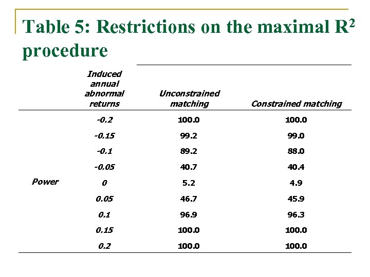
Table 5: Restrictions on the maximal R 2 procedure Induced annual abnormal returns Constrained matching -0. 2 100. 0 -0. 15 99. 2 99. 0 -0. 1 89. 2 88. 0 -0. 05 Power Unconstrained matching 40. 7 40. 4 0 5. 2 4. 9 0. 05 46. 7 45. 9 0. 1 96. 9 96. 3 0. 15 100. 0 0. 2 100. 0

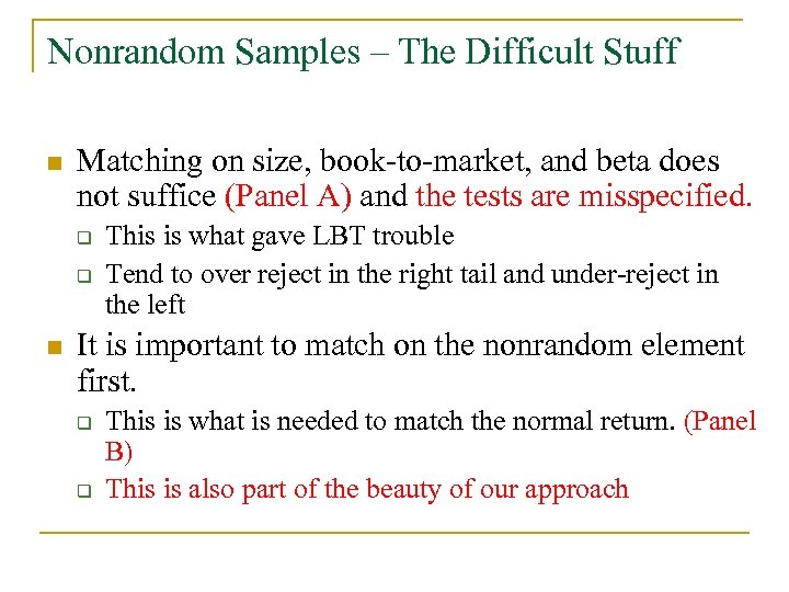
Nonrandom Samples – The Difficult Stuff n Matching on size, book-to-market, and beta does not suffice (Panel A) and the tests are misspecified. q q n This is what gave LBT trouble Tend to over reject in the right tail and under-reject in the left It is important to match on the nonrandom element first. q q This is what is needed to match the normal return. (Panel B) This is also part of the beauty of our approach

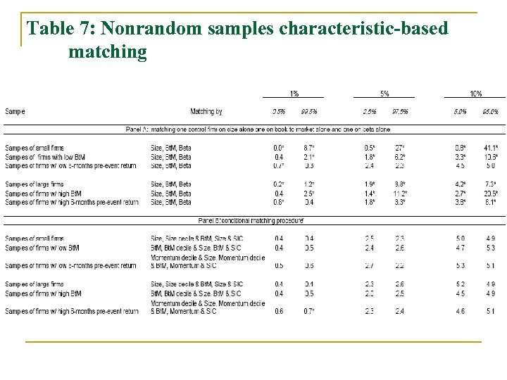
Table 7: Nonrandom samples characteristic-based matching

What About Contemporaneous Correlation? n Calendar clustering (see e. g. Mitchell and Stafford (2000)) can cause misspecification problems. q The issue is that stock returns are correlated crosssectionally. It may be that BHARs are as well. n n n If so, assuming independence means that the denominator in the test statistic is too small and rejection occurs too often. This could affect our tests as well. To check, we do simulations where event time and calendar time are the same. q The event date is the same for every sample firm.

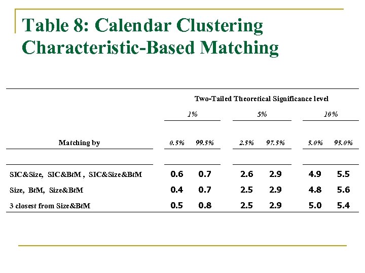
Table 8: Calendar Clustering Characteristic-Based Matching Two-Tailed Theoretical Significance level 1% 5% 10% Matching by 0. 5% 99. 5% 2. 5% 97. 5% 5. 0% 95. 0% SIC&Size, SIC&Bt. M , SIC&Size&Bt. M 0. 6 0. 7 2. 6 2. 9 4. 9 5. 5 Size, Bt. M, Size&Bt. M 0. 4 0. 7 2. 5 2. 9 4. 8 5. 6 3 closest from Size&Bt. M 0. 5 0. 8 2. 5 2. 9 5. 0 5. 4

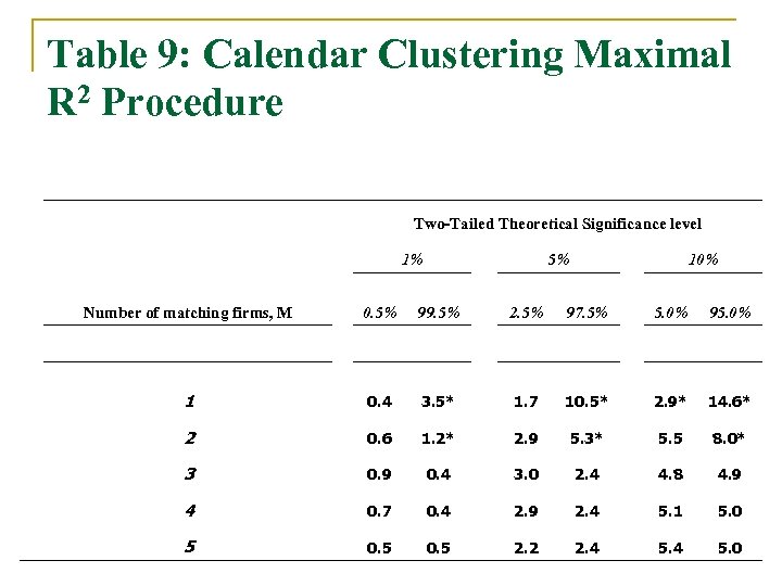
Table 9: Calendar Clustering Maximal R 2 Procedure Two-Tailed Theoretical Significance level 1% 5% 10% Number of matching firms, M 0. 5% 99. 5% 2. 5% 97. 5% 5. 0% 95. 0% 1 0. 4 3. 5* 1. 7 10. 5* 2. 9* 14. 6* 2 0. 6 1. 2* 2. 9 5. 3* 5. 5 8. 0* 3 0. 9 0. 4 3. 0 2. 4 4. 8 4. 9 4 0. 7 0. 4 2. 9 2. 4 5. 1 5. 0 5 0. 5 2. 2 2. 4 5. 0

Why might the test be correctly specified in the face of clustering? n The BHAR is the difference between two returns. q q Perhaps using the control firm approach means that the resulting BHARs have less cross sectional correlation because common components of idiosyncratic risk are removed by careful control firm choice. Using an index may fail because even if the asset pricing model is correct, only the systematic component of returns would be removed. n Average BHAR correlation using matching firms: . 002 -. 018 is the average reported by Mitchell and Stafford using the reference portfolio approach while our approach yields an average of. 00015

Further Robustness n Control firm selection q Remove noise by more closely matching the mean. n Match on two attributes at once. For example: § n n Size and book-to-market, book-to-market and industry, industry and size. This made little difference in random samples (Table 3). Will it improve things in the non-random sample procedure? Univariate regressions (unreported, reintroduced skewness) Is it the matching technology alone? q If you create a portfolio from the M matching firms and then use the empirical p-value, what happens (table 6)? n n Power is lower and the asymmetric power re-appears. Most of the increase in power appears to come from multiple control firm approach.

Still To Do n More on nonrandom samples q Induce more correlation n n Use our procedure and the CRSP Events dataset to consider the results for well examined events. q n Industry and time Work in progress. Horse races vs. the calendar time approach? n n Compare size and power of the tests. Different inference (measurement bias)