fb50f4b76d9f25c828dcff232ce39439.ppt
- Количество слайдов: 38
A Prediction-based Approach to Distributed Interactive Applications Peter A. Dinda Department of Computer Science Northwestern University http: //www. cs. nwu. edu/~pdinda
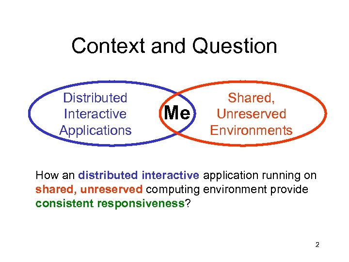
Context and Question Distributed Interactive Applications Me Shared, Unreserved Environments How an distributed interactive application running on shared, unreserved computing environment provide consistent responsiveness? 2
Why Is This Interesting? • Interactive resource demands exploding • Tools and toys increasingly are physical simulations • New kinds of resource-intensive applications • Responsiveness tied to peak demand • People provision according to peak demand • 90% of the time CPU or network link is unused • Opportunity to use the resources smarter • Build more powerful, more interesting apps • Shared resource pools, resource markets, The Grid… • Resource reservations unlikely • History argues against it, partial reservation, … 3
Approach • Soft real-time model • Responsiveness -> deadline • Advisory, no guarantees • Adaptation mechanisms • Exploit DOF available in environment • Prediction of resource supply and demand • Control the mechanisms to benefit the application • Avoid synchronization Rigorous statistical and systems approach to prediction 4
Outline • Distributed interactive applications • Image editing, scientific visualization, virtualized audio • • • Real-time scheduling advisors Running time advisor Resource signals RPS system Current work 5
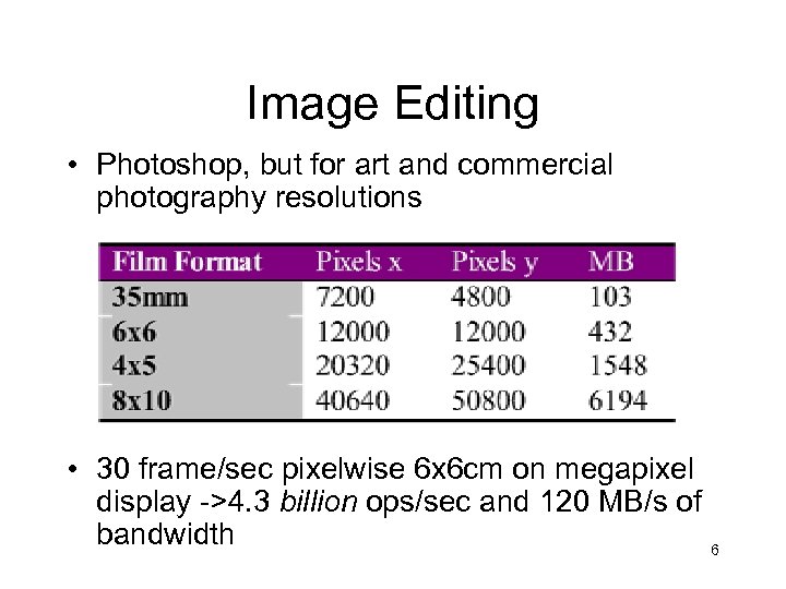
Image Editing • Photoshop, but for art and commercial photography resolutions • 30 frame/sec pixelwise 6 x 6 cm on megapixel display ->4. 3 billion ops/sec and 120 MB/s of bandwidth 6
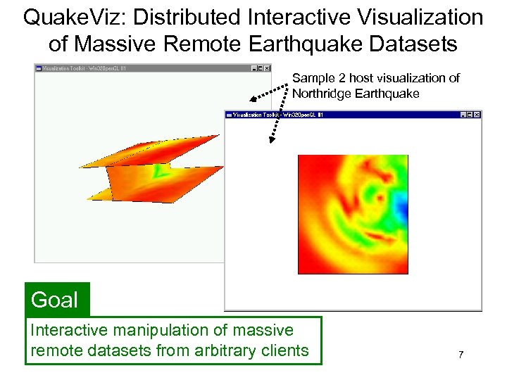
Quake. Viz: Distributed Interactive Visualization of Massive Remote Earthquake Datasets Sample 2 host visualization of Northridge Earthquake Goal Interactive manipulation of massive remote datasets from arbitrary clients 7
DV Framework For Distributed Interactive Visualization • Large datasets (e. g. , earthquake simulations) • Distributed VTK visualization pipelines • Active frames • • Encapsulate data, computation, path through pipeline Launched from server by user interaction Annotated with deadline Dynamically chose on which host each pipeline stage will execute and what quality settings to use http: //www. cs. cmu. edu/~dv 8
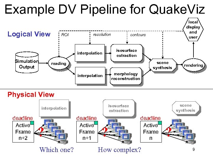
Example DV Pipeline for Quake. Viz Logical View ROI resolution interpolation Simulation Output local display and user contours isosurface extraction scene synthesis reading interpolation rendering morphology reconstruction Physical View deadline Active Frame n+2 ? Which one? scene synthesis isosurface extraction interpolation deadline Active Frame n+1 ? deadline Active Frame n How complex? ? 9
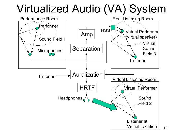
Virtualized Audio (VA) System 10
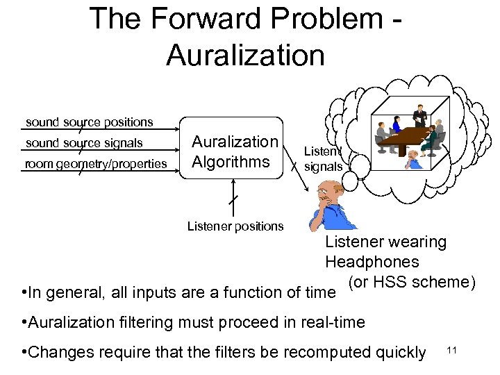
The Forward Problem Auralization sound source positions sound source signals room geometry/properties Auralization Algorithms Listener signals Listener positions Listener wearing Headphones (or HSS scheme) • In general, all inputs are a function of time • Auralization filtering must proceed in real-time • Changes require that the filters be recomputed quickly 11
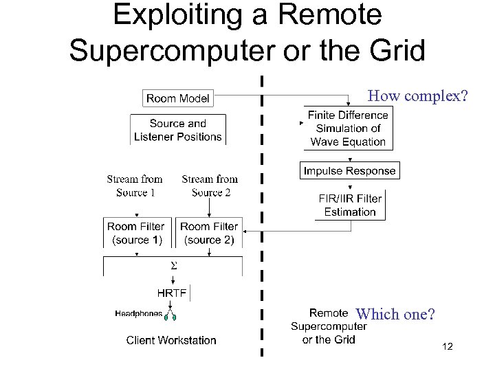
Exploiting a Remote Supercomputer or the Grid How complex? Which one? 12
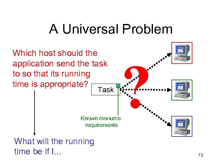
A Universal Problem Which host should the application send the task to so that its running time is appropriate? Task Known resource requirements What will the running time be if I. . . ? 13
Real-time Scheduling Advisor • Real-time for distributed interactive applications • Assumptions • • • Sequential tasks initiated by user actions Aperiodic arrivals Resilient deadlines (soft real-time) Compute-bound tasks Known computational requirements • Best-effort semantics • Recommend host where deadline is likely to be met • Predict running time on that host • No guarantees 14
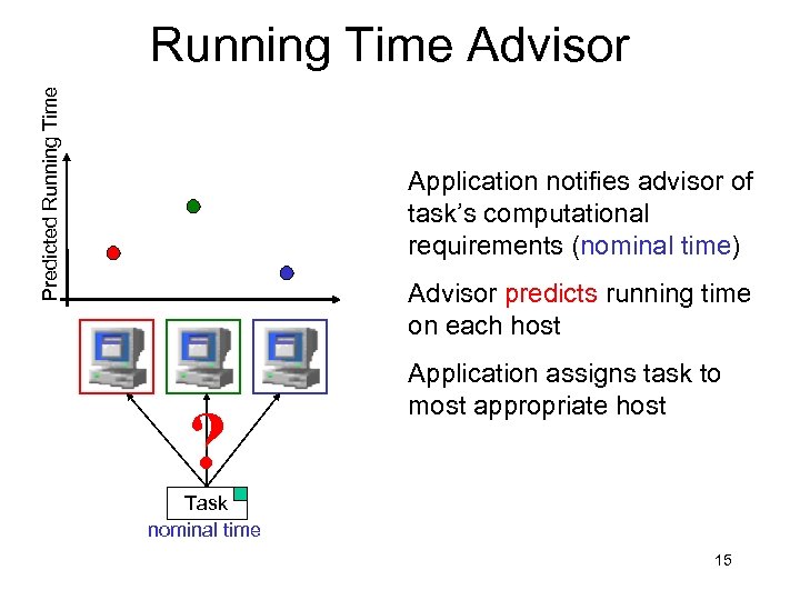
Predicted Running Time Advisor Application notifies advisor of task’s computational requirements (nominal time) Advisor predicts running time on each host ? Application assigns task to most appropriate host Task nominal time 15
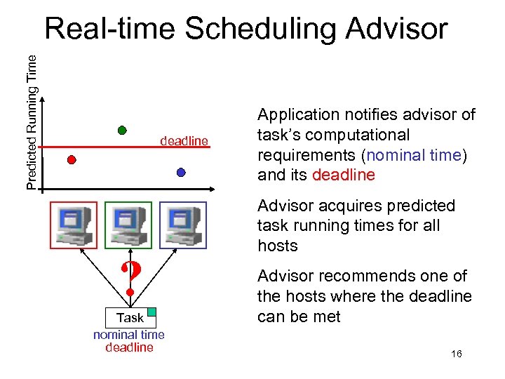
Predicted Running Time Real-time Scheduling Advisor deadline ? Task nominal time deadline Application notifies advisor of task’s computational requirements (nominal time) and its deadline Advisor acquires predicted task running times for all hosts Advisor recommends one of the hosts where the deadline can be met 16
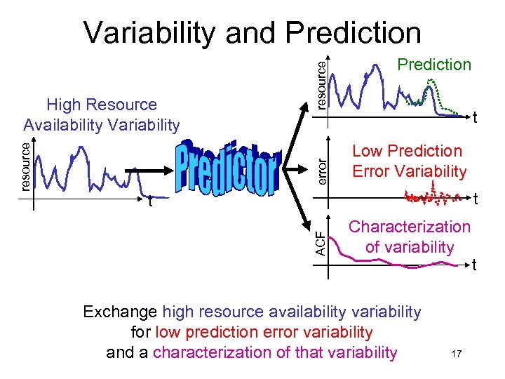
error Prediction t Low Prediction Error Variability t t ACF resource High Resource Availability Variability resource Variability and Prediction Characterization of variability Exchange high resource availability variability for low prediction error variability and a characterization of that variability 17 t
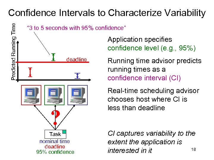
Predicted Running Time Confidence Intervals to Characterize Variability “ 3 to 5 seconds with 95% confidence” Application specifies confidence level (e. g. , 95%) deadline ? Task nominal time deadline 95% confidence Running time advisor predicts running times as a confidence interval (CI) Real-time scheduling advisor chooses host where CI is less than deadline CI captures variability to the extent the application is 18 interested in it
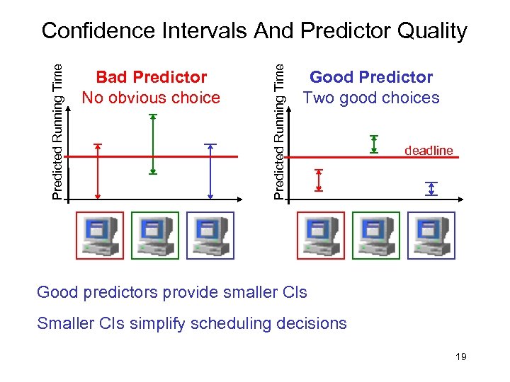
Bad Predictor No obvious choice Predicted Running Time Confidence Intervals And Predictor Quality Good Predictor Two good choices deadline Good predictors provide smaller CIs Smaller CIs simplify scheduling decisions 19
Overview of Research Results • Predicting CIs is feasible • Host load prediction using AR(16) models • Running time estimation using host load predictions • Predicting CIs is practical • RPS Toolkit (inc. in CMU Remos, BBN Qu. O) • Extremely low-overhead online system • Predicting CIs is useful • Performance of real-time scheduling advisor Measured performance of real system Statistically rigorous analysis and evaluation 20
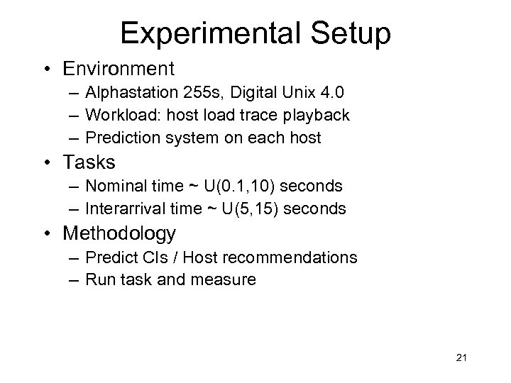
Experimental Setup • Environment – Alphastation 255 s, Digital Unix 4. 0 – Workload: host load trace playback – Prediction system on each host • Tasks – Nominal time ~ U(0. 1, 10) seconds – Interarrival time ~ U(5, 15) seconds • Methodology – Predict CIs / Host recommendations – Run task and measure 21
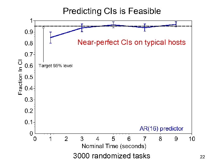
Predicting CIs is Feasible Near-perfect CIs on typical hosts 3000 randomized tasks 22
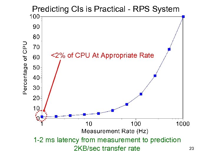
Predicting CIs is Practical - RPS System <2% of CPU At Appropriate Rate 1 -2 ms latency from measurement to prediction 2 KB/sec transfer rate 23
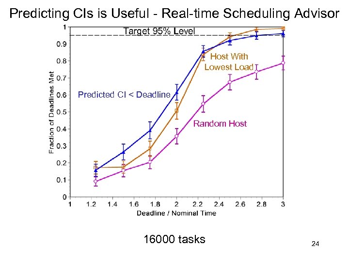
Predicting CIs is Useful - Real-time Scheduling Advisor Host With Lowest Load Predicted CI < Deadline Random Host 16000 tasks 24
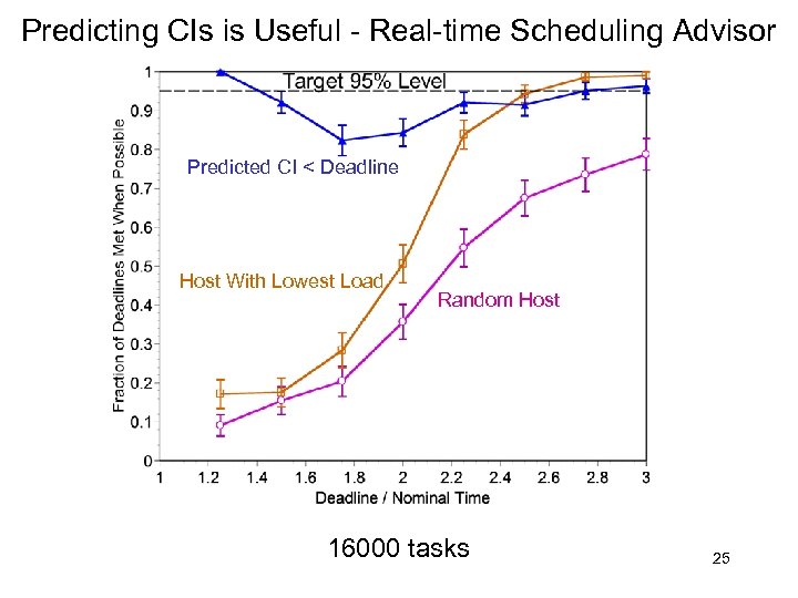
Predicting CIs is Useful - Real-time Scheduling Advisor Predicted CI < Deadline Host With Lowest Load Random Host 16000 tasks 25
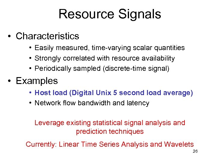
Resource Signals • Characteristics • Easily measured, time-varying scalar quantities • Strongly correlated with resource availability • Periodically sampled (discrete-time signal) • Examples • Host load (Digital Unix 5 second load average) • Network flow bandwidth and latency Leverage existing statistical signal analysis and prediction techniques Currently: Linear Time Series Analysis and Wavelets 26
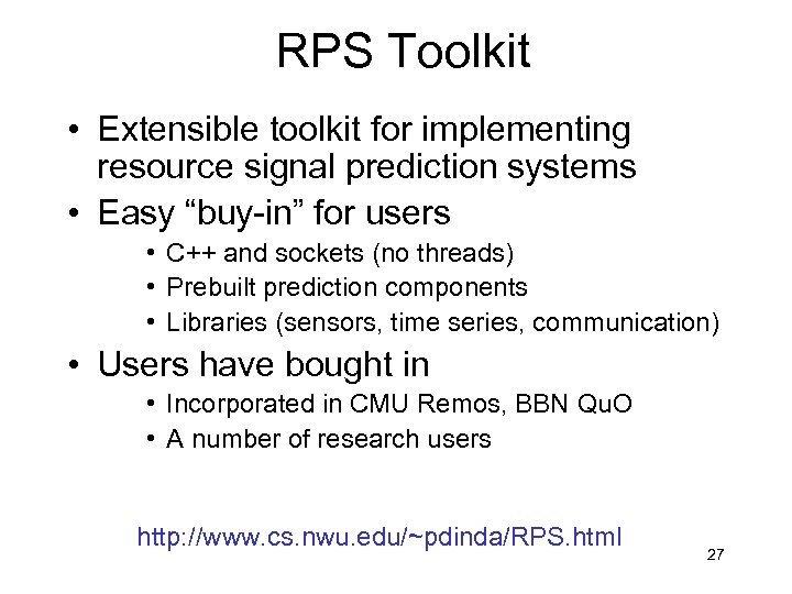
RPS Toolkit • Extensible toolkit for implementing resource signal prediction systems • Easy “buy-in” for users • C++ and sockets (no threads) • Prebuilt prediction components • Libraries (sensors, time series, communication) • Users have bought in • Incorporated in CMU Remos, BBN Qu. O • A number of research users http: //www. cs. nwu. edu/~pdinda/RPS. html 27
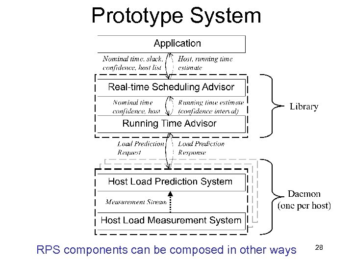
Prototype System RPS components can be composed in other ways 28
Limitations • Compute-intensive apps only • Host load based • Network prediction not solved • Not even limits are known • Poor scheduler models • Poor integration of resource supply predictions • Programmer supplies resource demand • Application resource demand prediction is nascent and needed 29
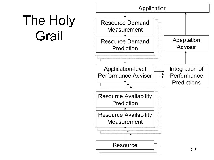
The Holy Grail 30
Current work • Wavelet-based techniques • Scalable information dissemination • Signal compression • Network prediction • Sampling theory and non-periodic sampling • Nonlinear predictive models • Better scheduler models • Relational approach to information • Proposal for Grid Forum Information Services Group • Application prediction • Activation trees 31
Conclusion • Prediction-based approach to responsive distributed interactive applications Peter Dinda, Jason Skicewicz, Dong Lu http: //www. cs. nwu. edu/~pdinda/RPS. html 32
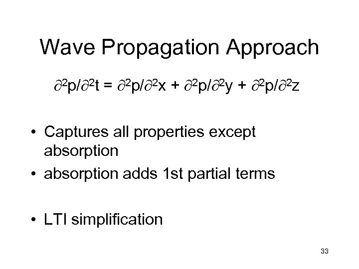
Wave Propagation Approach ¶ 2 p/¶ 2 t = ¶ 2 p/¶ 2 x + ¶ 2 p/¶ 2 y + ¶ 2 p/¶ 2 z • Captures all properties except absorption • absorption adds 1 st partial terms • LTI simplification 33
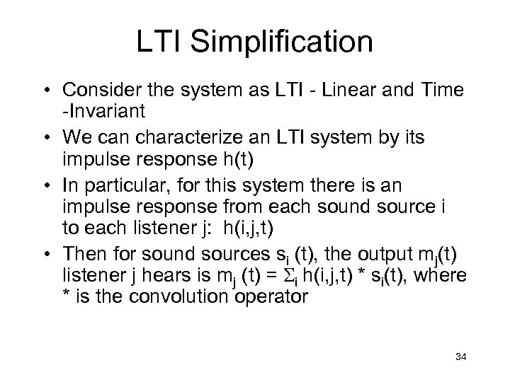
LTI Simplification • Consider the system as LTI - Linear and Time -Invariant • We can characterize an LTI system by its impulse response h(t) • In particular, for this system there is an impulse response from each sound source i to each listener j: h(i, j, t) • Then for sound sources si (t), the output mj(t) listener j hears is mj (t) = Si h(i, j, t) * si(t), where * is the convolution operator 34
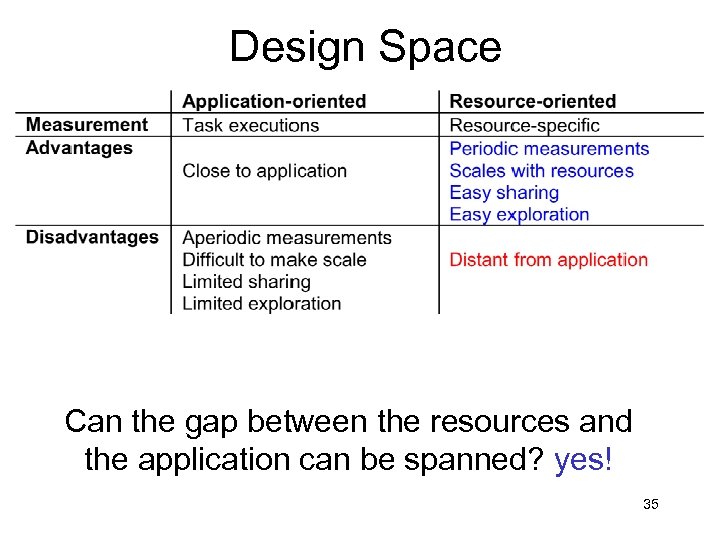
Design Space Can the gap between the resources and the application can be spanned? yes! 35
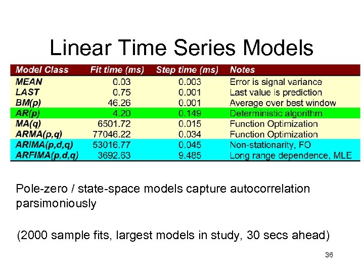
Linear Time Series Models Pole-zero / state-space models capture autocorrelation parsimoniously (2000 sample fits, largest models in study, 30 secs ahead) 36
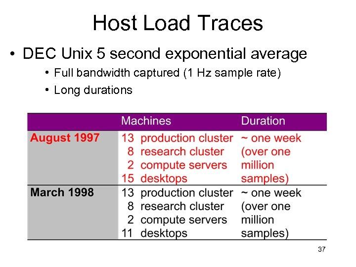
Host Load Traces • DEC Unix 5 second exponential average • Full bandwidth captured (1 Hz sample rate) • Long durations 37
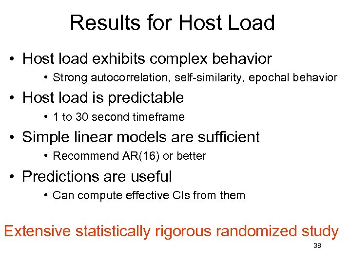
Results for Host Load • Host load exhibits complex behavior • Strong autocorrelation, self-similarity, epochal behavior • Host load is predictable • 1 to 30 second timeframe • Simple linear models are sufficient • Recommend AR(16) or better • Predictions are useful • Can compute effective CIs from them Extensive statistically rigorous randomized study 38
fb50f4b76d9f25c828dcff232ce39439.ppt