

Атмосфера.ppt
- Количество слайдов: 72
 A. N. Severtsov Institute of ecology and evolution RAS J. Kurbatova Experimental support and ecological monitoring models (C-fluxes).
 The Institute of ecology and evolution of the Russian Academy of") (http//www. sevin. ru) The Institute of ecology and evolution of the Russian Academy of Sciences established in 1934 by academician A. N. Severtsov is one of the leading biological institutes of Russia. The Institute is a scientific research centre on ecology, biological diversity, ethology, evolutionary morphology and nature conservation. The Principal Directions Of The Studies -Structural and functional organization, dynamics and evolution of populations, communities and ecosystems; -Ecology of organisms and mechanisms of adaptation; -Ecological and evolutionary aspects of animal behavior and communications; -Morphological regularities and mechanisms of animal evolution; -Biological diversity and sustainable use of biological resources. -Fundamental problems of nature conservation.
(http//www. sevin. ru) The Institute of ecology and evolution of the Russian Academy of Sciences established in 1934 by academician A. N. Severtsov is one of the leading biological institutes of Russia. The Institute is a scientific research centre on ecology, biological diversity, ethology, evolutionary morphology and nature conservation. The Principal Directions Of The Studies -Structural and functional organization, dynamics and evolution of populations, communities and ecosystems; -Ecology of organisms and mechanisms of adaptation; -Ecological and evolutionary aspects of animal behavior and communications; -Morphological regularities and mechanisms of animal evolution; -Biological diversity and sustainable use of biological resources. -Fundamental problems of nature conservation.
 Global climate changes
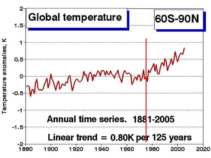
: - Eleven of the last") Глобальные климатические изменения Проявления глобального потепления климата (IPCC, 2007): - Eleven of the last twelve years (1995 -2006) rank among the twelve warmest years in the instrumental record of global surface temperature (since 1850). The 100 -year linear trend (1906 -2005) of 0. 74 [0. 56 to 0. 92]°C is larger than the corresponding trend of 0. 6 [0. 4 to 0. 8]°C (1901 -2000) given in the TAR (Figure 1. 1). The linear warming trend over the 50 years from 1956 to 2005 (0. 13 [0. 10 to 0. 16]°C per decade) is nearly twice that for the 100 years from 1906 to 2005. - Increases in sea level are consistent with warming. Global average sea level rose at an average rate of 1. 8 [1. 3 to 2. 3]mm per year over 1961 to 2003 and at an average rate of about 3. 1 [2. 4 to 3. 8]mm per year from 1993 to 2003. Observed decreases in snow and ice extent are also consistent with warming. Satellite data since 1978 show that annual average Arctic sea ice extent has shrunk by 2. 7 [2. 1 to 3. 3]% per decade, with larger decreases in summer of 7. 4 [5. 0 to 9. 8]% per decade.
Глобальные климатические изменения Проявления глобального потепления климата (IPCC, 2007): - Eleven of the last twelve years (1995 -2006) rank among the twelve warmest years in the instrumental record of global surface temperature (since 1850). The 100 -year linear trend (1906 -2005) of 0. 74 [0. 56 to 0. 92]°C is larger than the corresponding trend of 0. 6 [0. 4 to 0. 8]°C (1901 -2000) given in the TAR (Figure 1. 1). The linear warming trend over the 50 years from 1956 to 2005 (0. 13 [0. 10 to 0. 16]°C per decade) is nearly twice that for the 100 years from 1906 to 2005. - Increases in sea level are consistent with warming. Global average sea level rose at an average rate of 1. 8 [1. 3 to 2. 3]mm per year over 1961 to 2003 and at an average rate of about 3. 1 [2. 4 to 3. 8]mm per year from 1993 to 2003. Observed decreases in snow and ice extent are also consistent with warming. Satellite data since 1978 show that annual average Arctic sea ice extent has shrunk by 2. 7 [2. 1 to 3. 3]% per decade, with larger decreases in summer of 7. 4 [5. 0 to 9. 8]% per decade.
 since 1960") Changes in glacier volume (km 3) since 1960
Changes in glacier volume (km 3) since 1960
 Why C - fluxes? The global atmospheric concentration of CO 2 increased from a pre-industrial value of about 280 ppm to 379 ppm in 2005. The annual CO 2 concentration growth rate was larger during the last 10 years (1995 -2005 average: 1. 9 ppm per year) than it has been since the beginning of continuous direct atmospheric measurements (1960 -2005 average: 1. 4 ppm per year), although there is year-to year variability in growth rates.
 Why C- fluxes? An idealised model of the natural greenhouse effect
 The C evolution in ecosystems Photosynthesis Ecosystem respiration leaf Soil respiration Allocation stem Root Respiration Litter and SOM decomposition storage root Microbial community Stabilized SOM Loss by leaching, erosion
 Researches in ecosystems Experimental studies Field researches Analyses and classification of results Modeling studies
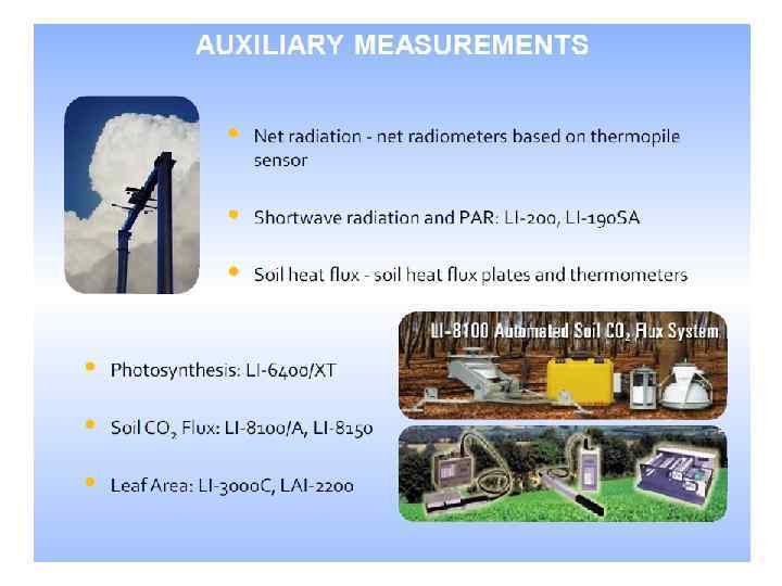
 Net radiation of forest ecosystem Sun radiation, S Reflected radiation Long wave radiation Of atmosphere, Ia Albedo (A) Long wave radiation of surface (IL) Rn=S-A+IA-IL
 Heat balance Net radiation Sensible and latent fluxes Heating Soil heat fluxes
 Water balance Precipitation evaporation
 CO 2 balance
 FLUXNET
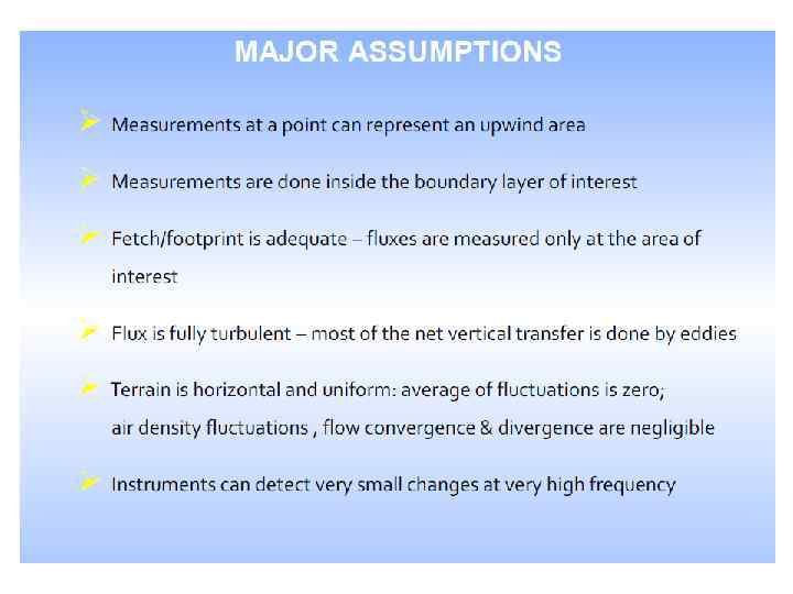
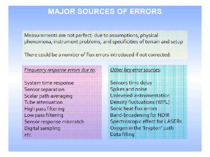
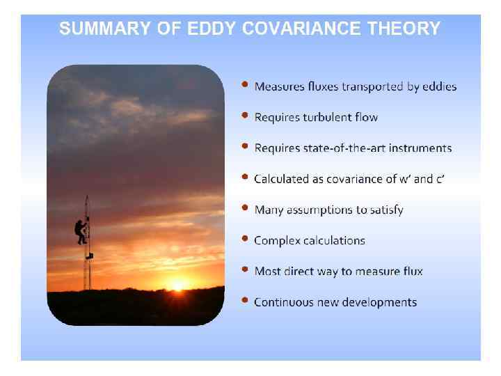
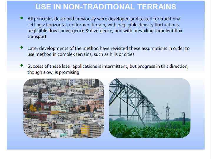
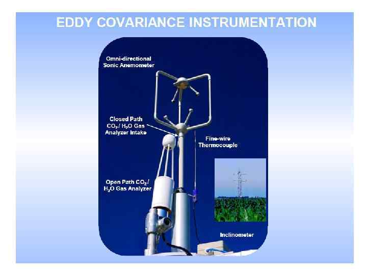
 EDDY COVARIANCE method Flux measurements State of methodology Air flow in ecosystems How to measure flux Derivation of main equation Major assumptions Major sources of errors Error treatment overview Use in non-traditional terrains Summary of EC theory
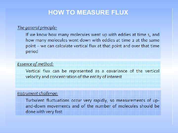
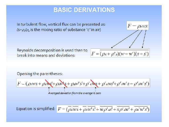
 WHAT IS FLUX? • Flux – how much of something moves through a unit area per unit time • Flux is dependent on: (1) number of things crossing the area; (2) size of the area being crossed, and (3) the time it takes to cross this area
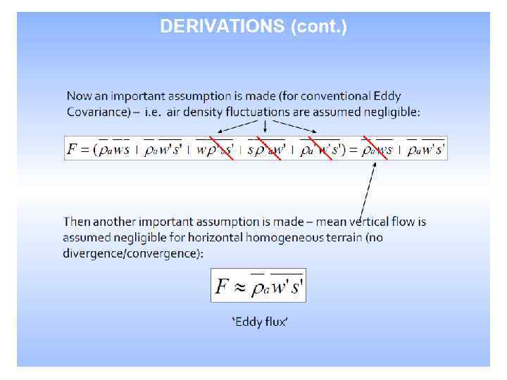
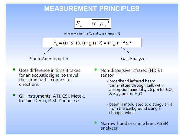
 FLUX MEASUREMENTS Flux measurements are widely used to estimate heat, water, and CO 2 exchange, as well as methane and other trace gases Eddy Covariance is one of the most direct and defensible ways to measure such fluxes The method is mathematically complex, and requires a lot of care setting up and processing data - but it is worth it!
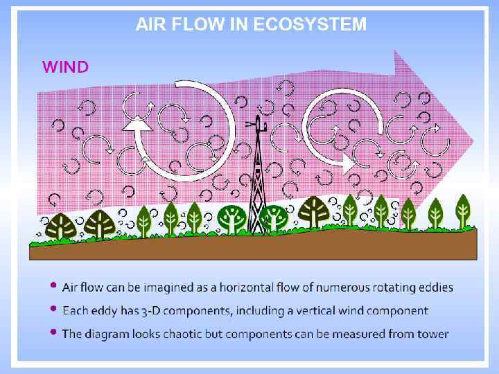
 WIND AIR FLOW IN ECOSYSTEM • Air flow can be imagined as a horizontal flow of numerous rotating eddies • Each eddy has 3 -D components, including a vertical wind component • The diagram looks chaotic but components can be measured from tower
 методы исследования Схема и основные датчики измерительного комплекса ФАР Измерительный комплекс Температура воздуха Скорость и направление ветра Потоки радиации 60 м Высокочастотные измерения скорости ветра Концентрация СО 2 и Н 2 О 40 м Давление Энергообеспечение Сохранение данных Газоанализатор Почвенное дыхание Осадки Уровень грунтовых вод Поток тепла в почву Температура почвы
 Eddy Covariance sites
 Объекты исследований Европейская часть России. Южная тайга 56°с. ш. , 33°в. д. Сфагновочерничный ельник (1998 - по н. в. ) Высота измерений 29 м Сложный ельник (1999 - по н. в. ) Высота измерений 44 м Верховое болото (1998 - 2000) Высота измерений 6 м
 Кумулятивные потоки диоксида углерода в южной тайге Европейской России: в лесу и на болоте bog
 Cat Tien. Vietnam. Soil flux measurements
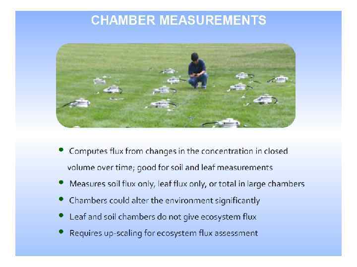
 Field observations Chamber methods + Li-COR
 Field observations Chambers
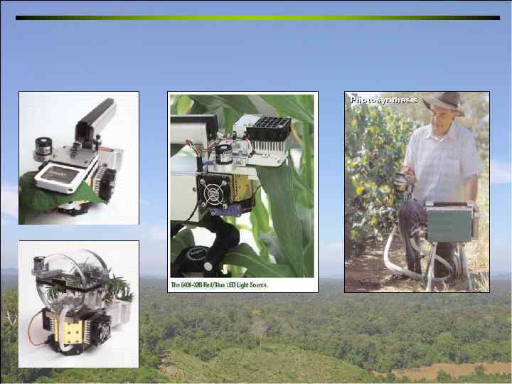
 Laboratory investigations
 Laboratory investigations
 Laboratory investigations
 Bioclimatological Modelling: Summary of achievements and perspectives for future research
 A variety of bioclimatological models: Empirical models, Statistical models, Process based models (describing biophysical and biochemical processes in plant canopy and soil).
 Bioclimatological process-based models: a key tool to describe land surface – atmosphere interaction in different spatial and temporal scales. Models of different levels of complexity: 1 D – 3 D , one- or multi-layer models; Time-step from 1 hour to 1 year Application: modelling of energy, H 2 O, CO 2, other trace gases exchange between land surface and the atmosphere (e. g. GCM, hydrological models); plant canopy growth and production; etc.
 Radiation balance equation: Energy balance equation: Water balance equation:
 Process-based approaches to describe the land surface - atmosphere interaction: ØThe first generation of the models e. g. the “bucket” models. ØBiophysical models: üRadiation absorption and spectral properties of the leaves, üTurbulent transfer, üBiophysical control of evapotranspiration (stomatal regulation), üPrecipitation interception and throughfall, üSoil moisture dynamics. ØCarbon cycle models. After Sellers et al. , Science, 1997
 Общая структура SVAT моделей
 1 -D models 2, 3 - D models
 1 -D model h 1 h 2 h 3 h 4 h. N d 1 d 2 d 3 d 4 d. N
.") Одномерные модели Описание растительности в виде нескольких слоев (однородных по горизонтали).
Одномерные модели Описание растительности в виде нескольких слоев (однородных по горизонтали).
 Achievements summary: local scale models 1 D models: Well developed both very simple and very sophisticated parameterisations of radiation, sensible heat, CO 2 fluxes, some trace gases within and above a plant canopy (mono or multi species). Soil water budget: still some uncertainties is available in e. g. definition of infiltration rate. Other problems: lack of input plant canopy parameters, a variety of biophysical properties
 2 - D structure of plants
 Achievements summary: local scale models 3 D models Well developed parameterisations: Leaf processes: radiation, transpiration, photosynthesis Canopy structure: analytical models, fractal geometry Solar radiation transfer in a plant canopy (short- and longwave radiation) with very fine resolution (Ross transfer equation, Monte Carlo approach). Turbulent transfer in a plant canopy (models of 1. 5 or high order closure) with resolution which exceeds at least by 10 times the resolution provided by radiation sub-model. Problems: lack of input parameters, large computing time
 Achievements summary: local scale models 3 D models of forest production and succession Models use well developed biological part, canopy structure, solar radiation transport. Nutrients transport in soil – plant system. Specificity: Low temporal resolution (in some models) for simulation of plant growth, mortality and vegetation type changes. Problems: parameterisation of water fluxes, …
 3 - D structure of plants N
 3 D structure -individual value
 Collecting model input parameters Global, regional and local scale models Application both land surface and remote sensing data Lack of input data especially for global and regional models Way to solve the problems: e. g. Sensitivity studies are required to select a most critical and important parameters for parameterisation of energy, water, CO 2, …. , fluxes (method: field and modelling studies e. g. in local scale)
 Availability of input meteorological parameters Meteorological parameters: Air temperature and humidity, Wind speed, Precipitation rate, CO 2 concentration, Global radiation, … e. g. Trace gas concentrations Regional scale: data from meteorological stations, mesoscale atmospheric model predictions Local scale: Measured or simulated meteorological data above a plant canopy usually within the atmospheric surface layer (not always available…. )
 Model validation Regional scale: Regional scale Measurements at key and representative plots, Cross-validation of modelling results, Measurement of total area fluxes e. g. catchment runoff for hydrological models … Local scale: long-term and short-term (field campaigns) Local scale: measurements at key representative plots, such micro-meteorological measurements, eddy flux measurements, soil and plant hydrology, … are required.
 scales (method, accuracy, …. ? )") Scalling up from point to grid (regional, global) scales (method, accuracy, …. ? )
Scalling up from point to grid (regional, global) scales (method, accuracy, …. ? )
 Общая структура региональной модели 1 -2. Пространственная интерполяция метеорологической информации в пределах исследуемой территории, и Реконструкция внутрисуточной изменчивости метеорологических параметров для ячеек регулярной сетки 3. Моделирование потоков тепла, Н 2 О и CO 2 для ячеек регулярной сетки в пределах исследуемой территории Радиационный Перенос перенос явного тепла 4. Интегрирование по пространству и времени потоков энергии, Н 2 О и СО 2 H 2 O перенос CO 2 перенос
 Perspectives for future modelling researches üDeeper process understanding and their explicit approximation (in leaf, plant canopy, soil); üPlant adaptation to changed environmental conditions (genetic and morphological); how to parameterise it? üTesting of principal model assumptions used in models and developing new algorithms and parameterisations; üApplication of new hypothesis and new measuring techniques for description and quantification of the parameters and processes in the models as well as for model validation (e. g. in remote sensing); üDeveloping alternative parameterisations…. .
 Perspectives for future researches Developing regional SVAT scale models should be well coupled with atmospheric models and well describe sub-grid heterogeneity; They should be use enough sophisticated and effective algorithm that allows to provide flux calculation using limited amount of key input parameters and without spent of a large amount of computer time.
 Perspectives for future researches Developing local 3 D scales SVAT models should be able to combine a very high spatial (for 3 D) and temporal resolution of a modelled ecosystem with enough sophisticated description of key SVAT processes. Integrating opportunity of the individual model describing some individual processes… may be with model describing economic and social development….
 и экспериментальных данных Институт исследования Земли, океанов и космоса,") Сравнение результатов численного моделирования (DNDC-модель) и экспериментальных данных Институт исследования Земли, океанов и космоса, Нью Хемпшир (США)
Сравнение результатов численного моделирования (DNDC-модель) и экспериментальных данных Институт исследования Земли, океанов и космоса, Нью Хемпшир (США)
 Спасибо за внимание