92854f0f5870bc3c5d2d356ad1bf24e3.ppt
- Количество слайдов: 61
 A Mesh-free Numerical Method for three-dimensional Nonlinear Schrödinger Equation Department of Computer Science and Information Systems Birkbeck, University of London Thomas C. L. Yue tclyue@gmail. com Feb 09, 2011 1
 Overview • Physical motivation of the problem – Dimensionless Gross-Pitaevskii equation (GPE) • Introduction to Radial basis functions (RBF) – Global supported strictly positive definite radial basis functions – Compactly supported radial basis funtions – Kansa’s method (asymmetric collocation) • Meshfree solution of cubic Nonlinear Schrodinger Equation – Numerical experiments and validation 2
 Physical Motivation 3
![Physical Motivation History of Bose Einstein Condensation (BEC) [1, 2] • First predicted by Physical Motivation History of Bose Einstein Condensation (BEC) [1, 2] • First predicted by](https://present5.com/presentation/92854f0f5870bc3c5d2d356ad1bf24e3/image-4.jpg) Physical Motivation History of Bose Einstein Condensation (BEC) [1, 2] • First predicted by Bose & Einstein (1924) • Experimentally observed in University of Colorado JILA lab (1995) What is BEC? [1, 2] • A phase of matter where all particles occupy the same quantum state • Occurs when diulated bosons (integer spin particles) gas are cooled to extremely low temperature (10 -9 K) • Individual particle wave functions behave as a single wave function 4
Physical Motivation History of Bose Einstein Condensation (BEC) [1, 2] • First predicted by Bose & Einstein (1924) • Experimentally observed in University of Colorado JILA lab (1995) What is BEC? [1, 2] • A phase of matter where all particles occupy the same quantum state • Occurs when diulated bosons (integer spin particles) gas are cooled to extremely low temperature (10 -9 K) • Individual particle wave functions behave as a single wave function 4
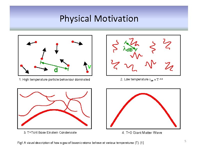 Physical Motivation 1. High temperature particle behaviour dominated 3. T=Tcrit Bose Einstein Condensate 2. Low temperature λd. B α T -0. 5 4. T=0 Giant Matter Wave Fig 1. A visual description of how a gas of bosonic-atoms behave at various temperatures (T). [1] 5
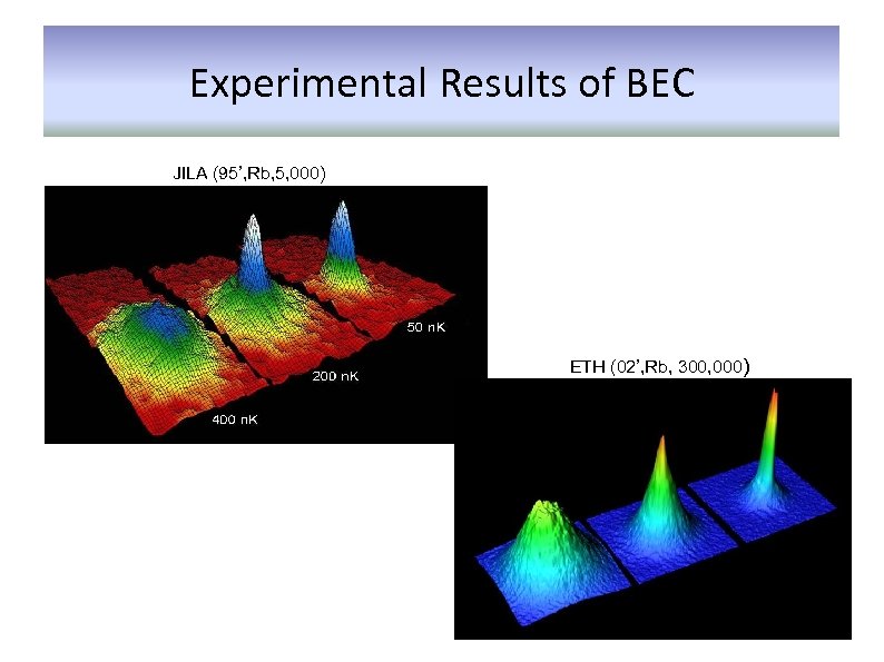 Experimental Results of BEC JILA (95’, Rb, 5, 000) ETH (02’, Rb, 300, 000)
![Gross–Pitaevskii equation • Hartree–Fock approximation [1, 2] – The many-body wavefunction is written as Gross–Pitaevskii equation • Hartree–Fock approximation [1, 2] – The many-body wavefunction is written as](https://present5.com/presentation/92854f0f5870bc3c5d2d356ad1bf24e3/image-7.jpg) Gross–Pitaevskii equation • Hartree–Fock approximation [1, 2] – The many-body wavefunction is written as productsof individual wave functions of each bosons [1, 2] • The Hamiltonian • The conserved quantities
Gross–Pitaevskii equation • Hartree–Fock approximation [1, 2] – The many-body wavefunction is written as productsof individual wave functions of each bosons [1, 2] • The Hamiltonian • The conserved quantities
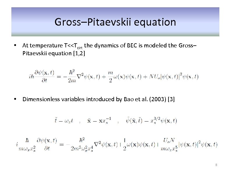 Gross–Pitaevskii equation • At temperature T<
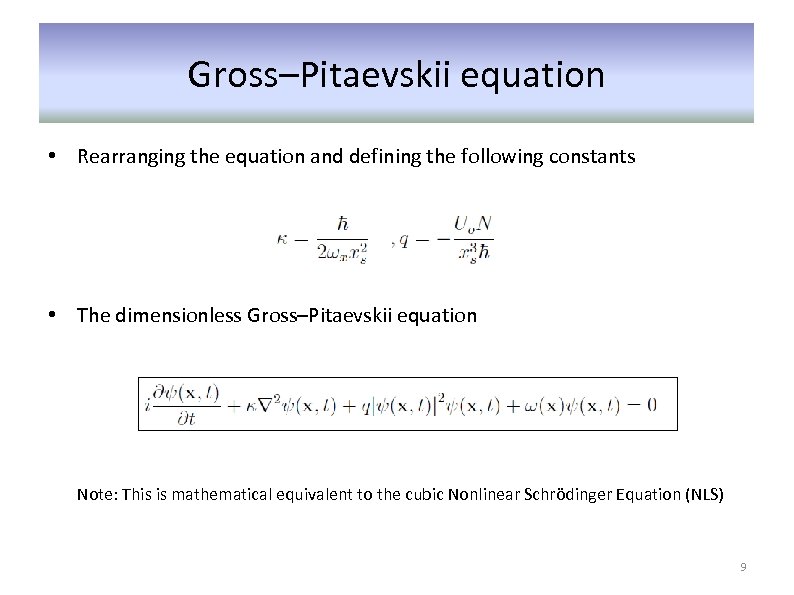 Gross–Pitaevskii equation • Rearranging the equation and defining the following constants • The dimensionless Gross–Pitaevskii equation Note: This is mathematical equivalent to the cubic Nonlinear Schrödinger Equation (NLS) 9
 Existing numerical methods for Nonlinear Schrödinger Equation Existing numerical methods for NLS Spectral Methods – Pseudo-spectral method (Muruganandam et al) – Time splitting Fourier spectral approximation (Bao et al. ) – Split-step Fourier spectral method (Weideman) Mesh-based Methods – Galerkin spectral (Dion et al. ) – Finite Element (Carl Joachim, Berdal Haga) – Split-step finite difference method (Wang) 10
 Existing numerical methods for Nonlinear Schrödinger Equation Existing numerical methods for NLS Spectral Methods – Pseudo-spectral method (Muruganandam et al) – Time splitting Fourier spectral approximation (Bao et al. ) – Split-step Fourier spectral method (Weideman) Mesh-based Methods – Galerkin spectral (Dion et al. ) – Finite Element (Carl Joachim, Berdal Haga) – Split-step finite difference method (Wang) Require mesh generation and re -meshing 11
 Radial Basis Functions 12
![Radial basis function • What is a radial basis function (RBF)? [4, 5] 13 Radial basis function • What is a radial basis function (RBF)? [4, 5] 13](https://present5.com/presentation/92854f0f5870bc3c5d2d356ad1bf24e3/image-13.jpg) Radial basis function • What is a radial basis function (RBF)? [4, 5] 13
Radial basis function • What is a radial basis function (RBF)? [4, 5] 13
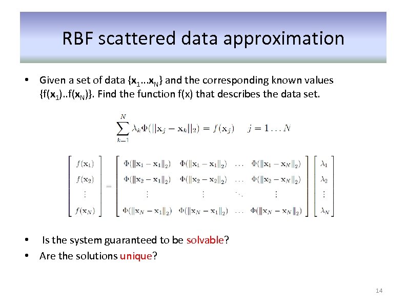 RBF scattered data approximation • Given a set of data {x 1. . . x. N} and the corresponding known values {f(x 1). . f(x. N)}. Find the function f(x) that describes the data set. • Is the system guaranteed to be solvable? • Are the solutions unique? 14
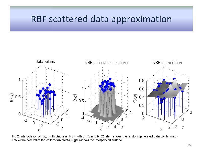 RBF scattered data approximation Fig 2. Interpolation of f(x, y) with Gaussian RBF with c=1/3 and N=25. (left) shows the random generated data points, (mid) shows the centred at the collocation points, (right) shows the interpolated surface. 15
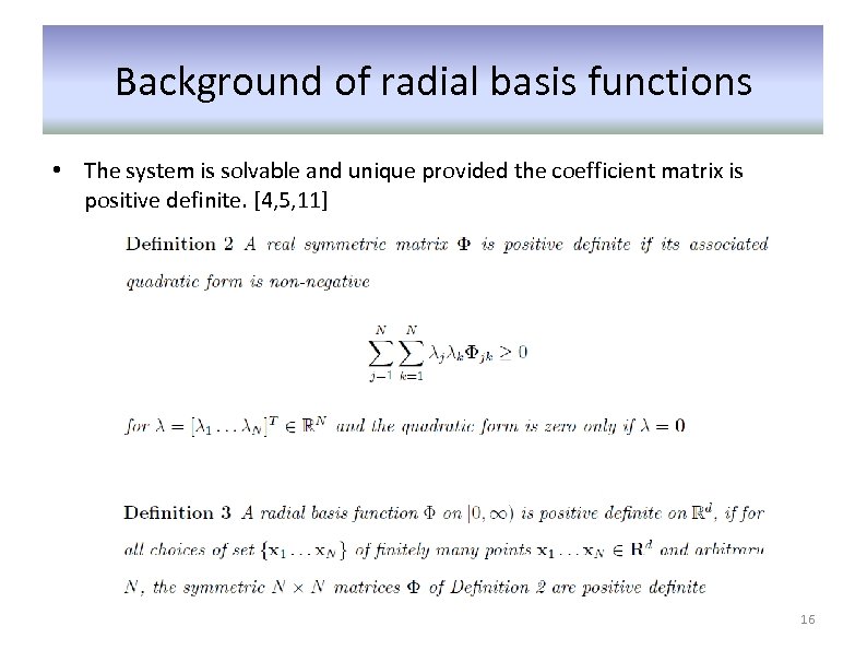 Background of radial basis functions • The system is solvable and unique provided the coefficient matrix is positive definite. [4, 5, 11] 16
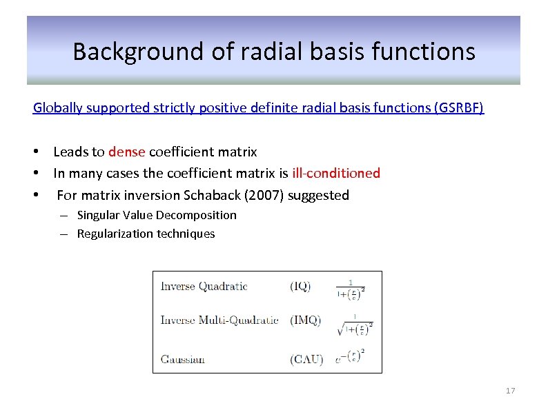 Background of radial basis functions Globally supported strictly positive definite radial basis functions (GSRBF) • Leads to dense coefficient matrix • In many cases the coefficient matrix is ill-conditioned • For matrix inversion Schaback (2007) suggested – Singular Value Decomposition – Regularization techniques 17
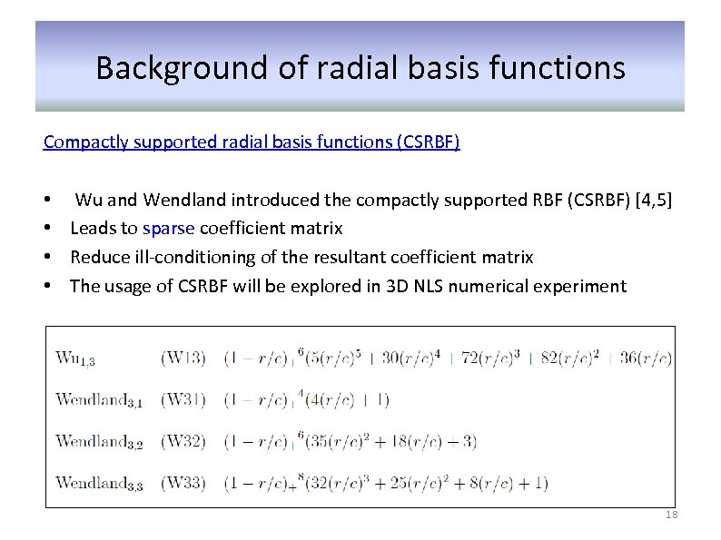 Background of radial basis functions Compactly supported radial basis functions (CSRBF) • • Wu and Wendland introduced the compactly supported RBF (CSRBF) [4, 5] Leads to sparse coefficient matrix Reduce ill-conditioning of the resultant coefficient matrix The usage of CSRBF will be explored in 3 D NLS numerical experiment 18
![Error Behaviour of RBF techniques • Trade off principle Schaback (1995) [5] Theorem: It Error Behaviour of RBF techniques • Trade off principle Schaback (1995) [5] Theorem: It](https://present5.com/presentation/92854f0f5870bc3c5d2d356ad1bf24e3/image-19.jpg) Error Behaviour of RBF techniques • Trade off principle Schaback (1995) [5] Theorem: It is impossible to construct radial basis functions which guarantees good stability and small errors at the same time. • Driscoll and Fornberg (2002) observed the "Flat Limit” [6] c->∞ leads to highly ill-conditioned RBF interpolation matrix c->0 implies highly localized RBFs such that it fails to approximate data between collocation points 19
Error Behaviour of RBF techniques • Trade off principle Schaback (1995) [5] Theorem: It is impossible to construct radial basis functions which guarantees good stability and small errors at the same time. • Driscoll and Fornberg (2002) observed the "Flat Limit” [6] c->∞ leads to highly ill-conditioned RBF interpolation matrix c->0 implies highly localized RBFs such that it fails to approximate data between collocation points 19
![Error Behaviour of RBF techniques • Wright, Fornberg, Larsson (2004) [7] – With increasing Error Behaviour of RBF techniques • Wright, Fornberg, Larsson (2004) [7] – With increasing](https://present5.com/presentation/92854f0f5870bc3c5d2d356ad1bf24e3/image-20.jpg) Error Behaviour of RBF techniques • Wright, Fornberg, Larsson (2004) [7] – With increasing shape parameter, interpolation error decreases sharply until the minimum numerical error is reached. – For any increasing shape parameter, interpolation error rapidly increases. The rapid decrease of interpolation error reaches a minimum. 20
Error Behaviour of RBF techniques • Wright, Fornberg, Larsson (2004) [7] – With increasing shape parameter, interpolation error decreases sharply until the minimum numerical error is reached. – For any increasing shape parameter, interpolation error rapidly increases. The rapid decrease of interpolation error reaches a minimum. 20
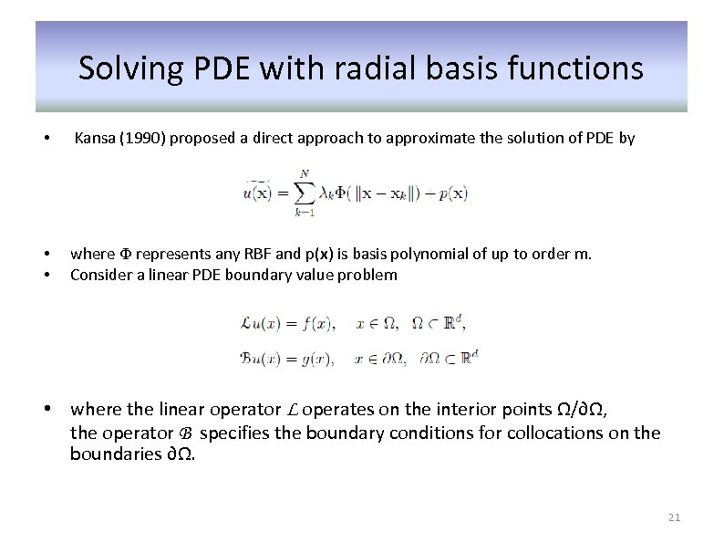 Solving PDE with radial basis functions • Kansa (1990) proposed a direct approach to approximate the solution of PDE by • • where Ф represents any RBF and p(x) is basis polynomial of up to order m. Consider a linear PDE boundary value problem • where the linear operator L operates on the interior points Ω/∂Ω, the operator B specifies the boundary conditions for collocations on the boundaries ∂Ω. 21
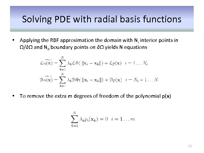 Solving PDE with radial basis functions • Applying the RBF approximation the domain with Ni interior points in Ω/∂Ω and Nb boundary points on ∂Ω yields N equations • To remove the extra m degrees of freedom of the polynomial p(x) 22
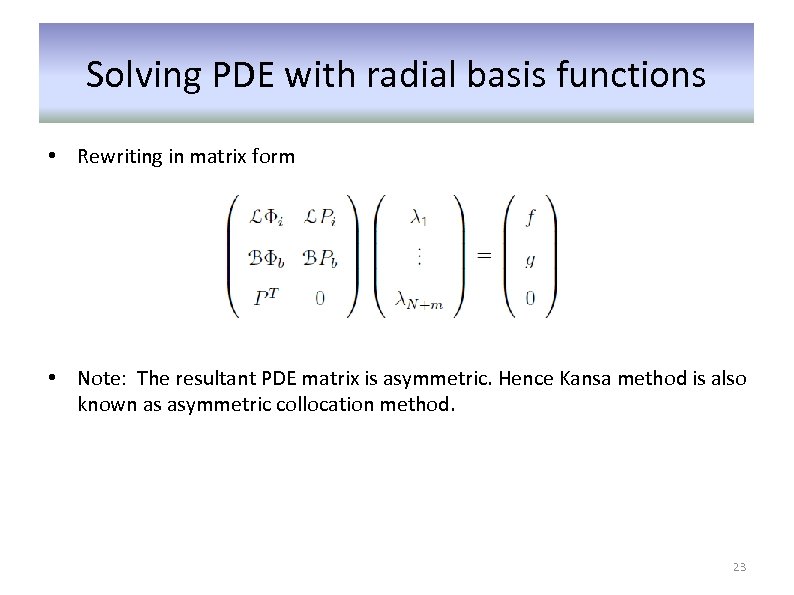 Solving PDE with radial basis functions • Rewriting in matrix form • Note: The resultant PDE matrix is asymmetric. Hence Kansa method is also known as asymmetric collocation method. 23
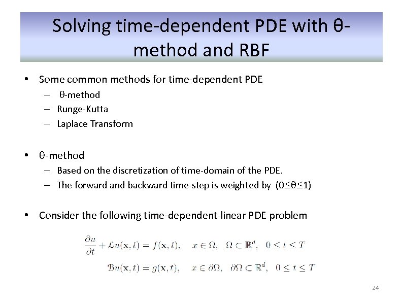 Solving time-dependent PDE with θmethod and RBF • Some common methods for time-dependent PDE – θ-method – Runge-Kutta – Laplace Transform • θ-method – Based on the discretization of time-domain of the PDE. – The forward and backward time-step is weighted by (0≤θ≤ 1) • Consider the following time-dependent linear PDE problem 24
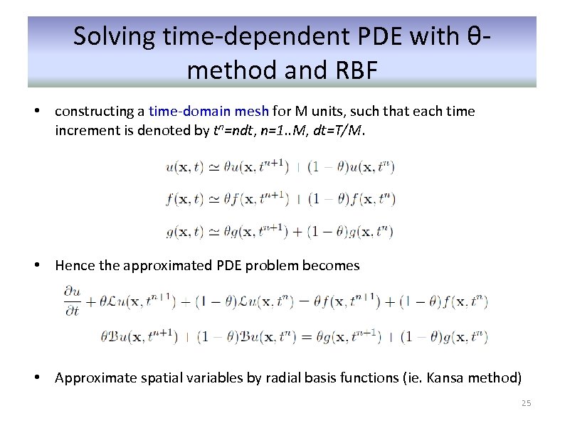 Solving time-dependent PDE with θmethod and RBF • constructing a time-domain mesh for M units, such that each time increment is denoted by tn=ndt, n=1. . M, dt=T/M. • Hence the approximated PDE problem becomes • Approximate spatial variables by radial basis functions (ie. Kansa method) 25
 Meshfree Numerical Method for Nonlinear Schrödinger Equation 26
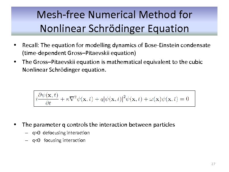 Mesh-free Numerical Method for Nonlinear Schrödinger Equation • Recall: The equation for modelling dynamics of Bose-Einstein condensate (time-dependent Gross–Pitaevskii equation) • The Gross–Pitaevskii equation is mathematical equivalent to the cubic Nonlinear Schrödinger equation. • The parameter q controls the interaction between particles – q>0 defocusing interaction – q<0 focusing interaction 27
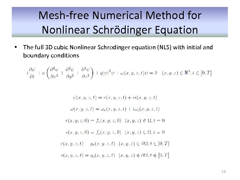 Mesh-free Numerical Method for Nonlinear Schrödinger Equation • The full 3 D cubic Nonlinear Schrodinger equation (NLS) with initial and boundary conditions 28
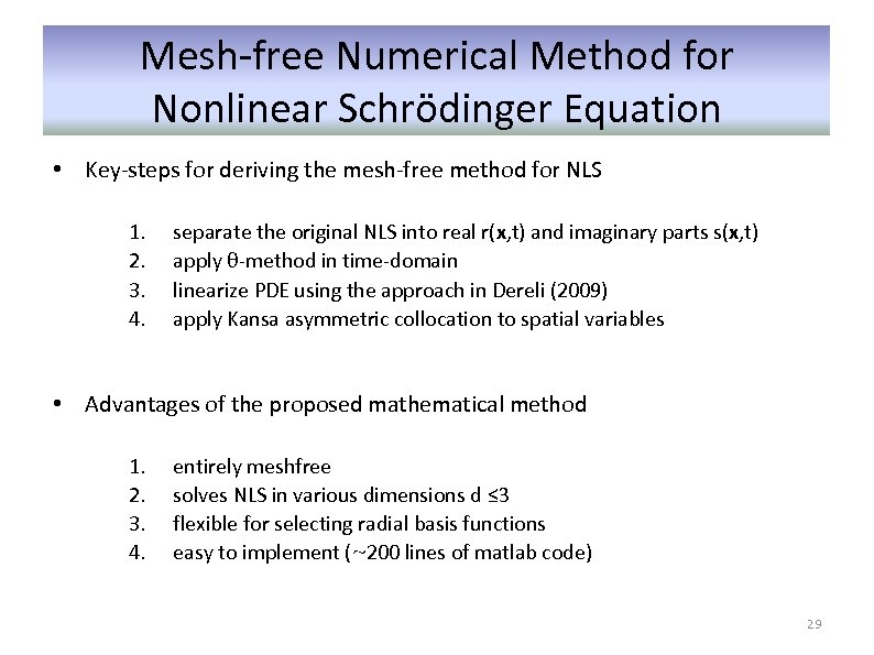 Mesh-free Numerical Method for Nonlinear Schrödinger Equation • Key-steps for deriving the mesh-free method for NLS 1. 2. 3. 4. separate the original NLS into real r(x, t) and imaginary parts s(x, t) apply θ-method in time-domain linearize PDE using the approach in Dereli (2009) apply Kansa asymmetric collocation to spatial variables • Advantages of the proposed mathematical method 1. 2. 3. 4. entirely meshfree solves NLS in various dimensions d ≤ 3 flexible for selecting radial basis functions easy to implement (~200 lines of matlab code) 29
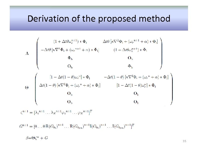
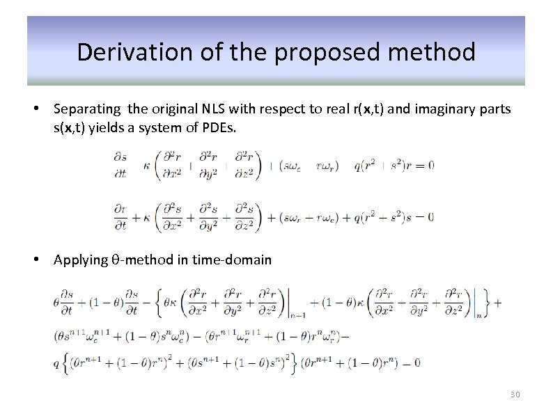 Derivation of the proposed method • Separating the original NLS with respect to real r(x, t) and imaginary parts s(x, t) yields a system of PDEs. • Applying θ-method in time-domain 30
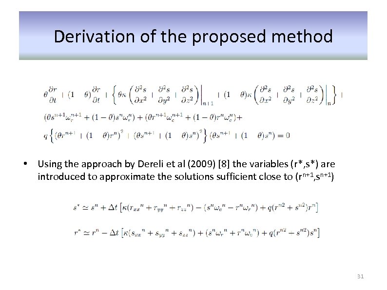 Derivation of the proposed method • Using the approach by Dereli et al (2009) [8] the variables (r*, s*) are introduced to approximate the solutions sufficient close to (rn+1, sn+1) 31
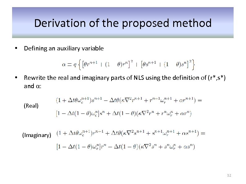 Derivation of the proposed method • Defining an auxiliary variable • Rewrite the real and imaginary parts of NLS using the definition of (r*, s*) and α: (Real) (Imaginary) 32
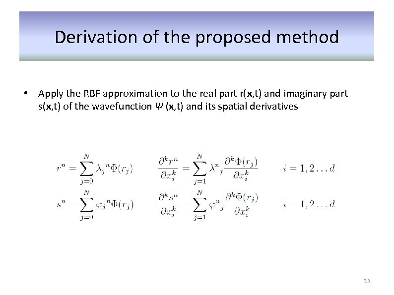 Derivation of the proposed method • Apply the RBF approximation to the real part r(x, t) and imaginary part s(x, t) of the wavefunction Ψ (x, t) and its spatial derivatives 33
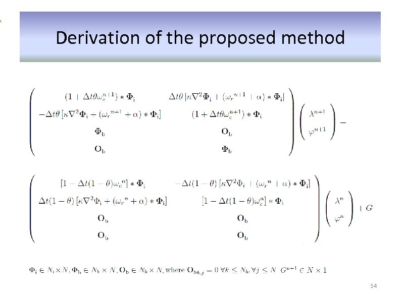 Derivation of the proposed method 34
 Derivation of the proposed method 35
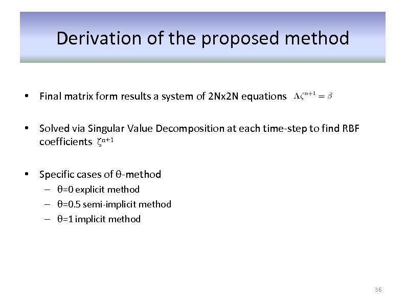 Derivation of the proposed method • Final matrix form results a system of 2 Nx 2 N equations • Solved via Singular Value Decomposition at each time-step to find RBF coefficients ζn+1 • Specific cases of θ-method – θ=0 explicit method – θ=0. 5 semi-implicit method – θ=1 implicit method 36
 Implementation flow-chart start Set up physical geometries and potential function Compute initial conditions Kernel of the method while t
 Numerical Experiments 38
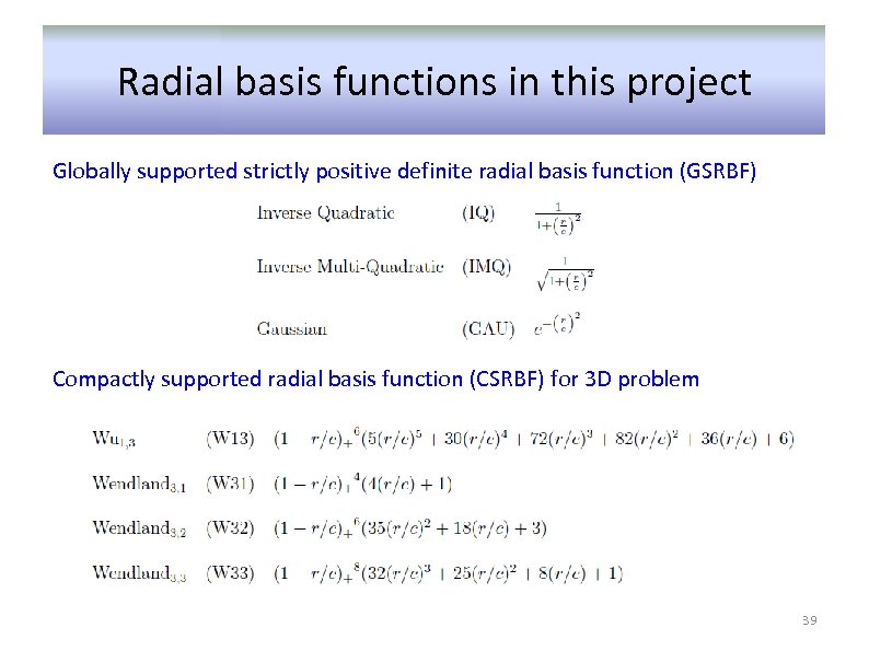 Radial basis functions in this project Globally supported strictly positive definite radial basis function (GSRBF) Compactly supported radial basis function (CSRBF) for 3 D problem 39
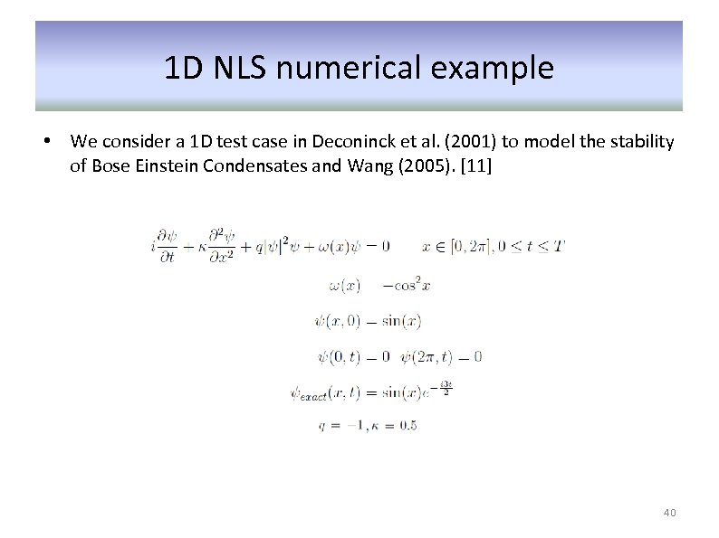 1 D NLS numerical example • We consider a 1 D test case in Deconinck et al. (2001) to model the stability of Bose Einstein Condensates and Wang (2005). [11] 40
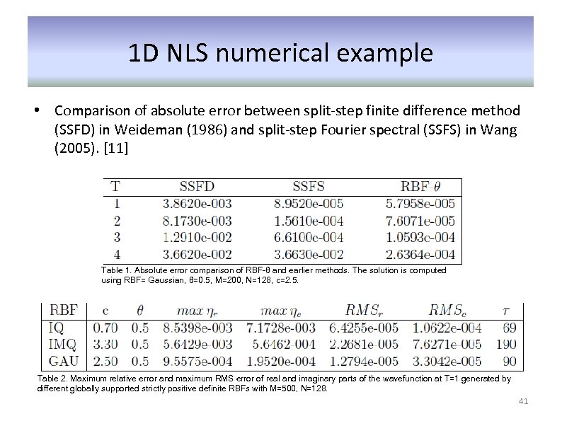 1 D NLS numerical example • Comparison of absolute error between split-step finite difference method (SSFD) in Weideman (1986) and split-step Fourier spectral (SSFS) in Wang (2005). [11] Table 1. Absolute error comparison of RBF-θ and earlier methods. The solution is computed using RBF= Gaussian, θ=0. 5, M=200, N=128, c=2. 5. Table 2. Maximum relative error and maximum RMS error of real and imaginary parts of the wavefunction at T=1 generated by different globally supported strictly positive definite RBFs with M=500, N=128. 41
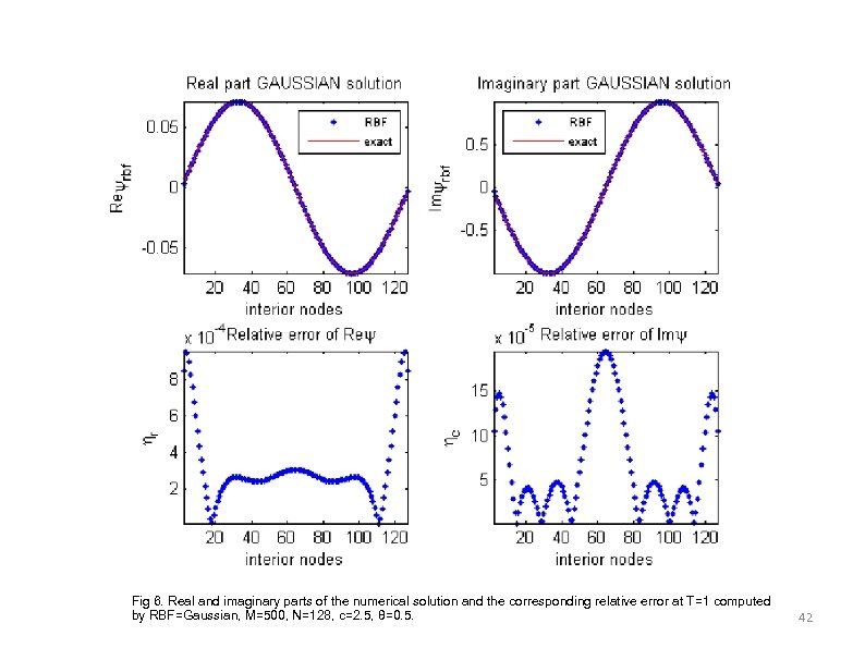 Fig 6. Real and imaginary parts of the numerical solution and the corresponding relative error at T=1 computed by RBF=Gaussian, M=500, N=128, c=2. 5, θ=0. 5. 42
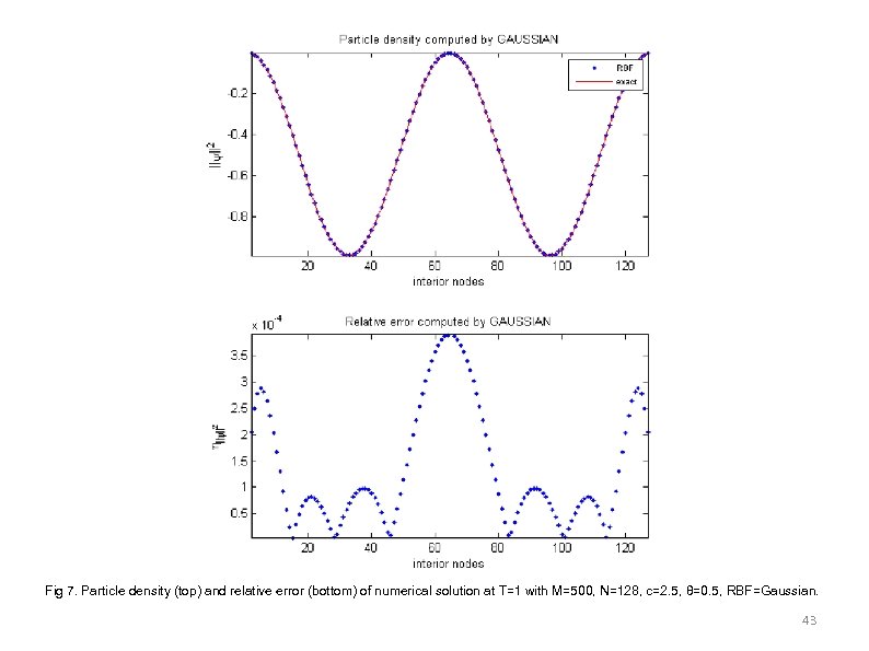 Fig 7. Particle density (top) and relative error (bottom) of numerical solution at T=1 with M=500, N=128, c=2. 5, θ=0. 5, RBF=Gaussian. 43
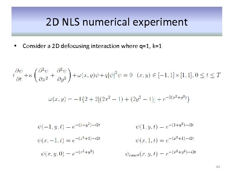 2 D NLS numerical experiment • Consider a 2 D defocusing interaction where q=1, k=1 44
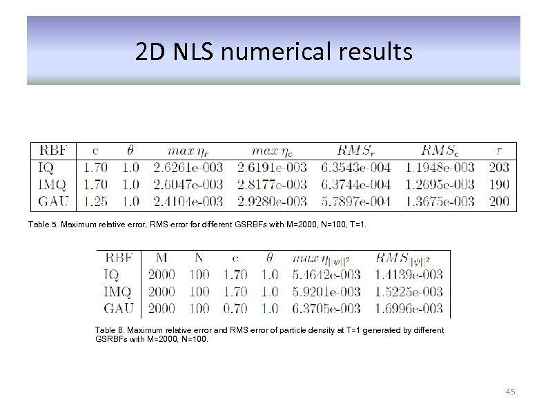 2 D NLS numerical results Table 5. Maximum relative error, RMS error for different GSRBFs with M=2000, N=100, T=1. Table 6. Maximum relative error and RMS error of particle density at T=1 generated by different GSRBFs with M=2000, N=100. 45
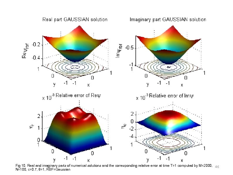 Fig 10. Real and imaginary parts of numerical solutions and the corresponding relative error at time T=1 computed by M=2000, 46 N=100, c=0. 7, θ=1, RBF=Gaussian
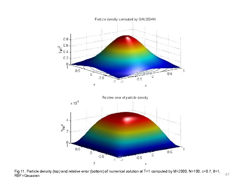 Fig 11. Particle density (top) and relative error (bottom) of numerical solution at T=1 computed by M=2000, N=100, c=0. 7, θ=1, RBF=Gaussian 47
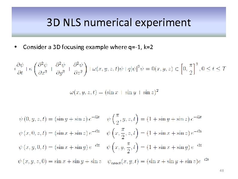 3 D NLS numerical experiment • Consider a 3 D focusing example where q=-1, k=2 48
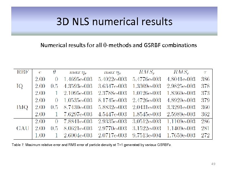 3 D NLS numerical results Numerical results for all θ-methods and GSRBF combinations Table 7. Maximum relative error and RMS error of particle density at T=1 generated by various GSRBFs. 49
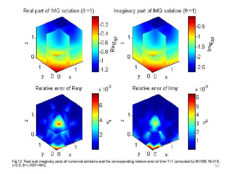 Fig 12. Real and imaginary parts of numerical solutions and the corresponding relative error at time T=1 computed by M=800, N=216, c=2. 0, θ=1, RBF=IMQ. 50
 3 D NLS numerical results Numerical results for all θ-methods and GSRBF combinations Table 7. Maximum relative error and RMS error of particle density at T=1 generated by various GSRBFs. 51
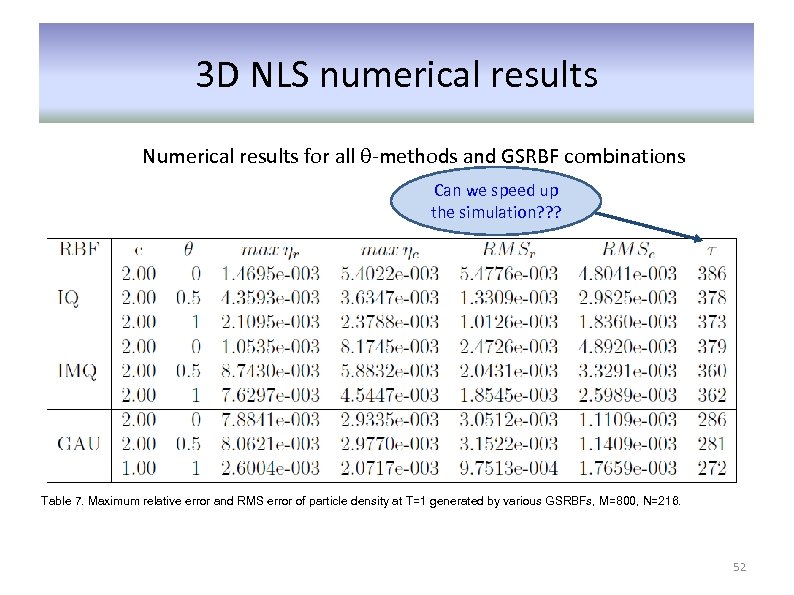 3 D NLS numerical results Numerical results for all θ-methods and GSRBF combinations Can we speed up the simulation? ? ? Table 7. Maximum relative error and RMS error of particle density at T=1 generated by various GSRBFs, M=800, N=216. 52
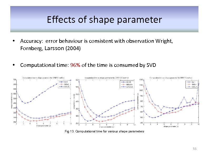 Effects of shape parameter • Accuracy: error behaviour is consistent with observation Wright, Fornberg, Larsson (2004) • Computational time: 96% of the time is consumed by SVD Fig 13. Computational time for various shape parameters 53
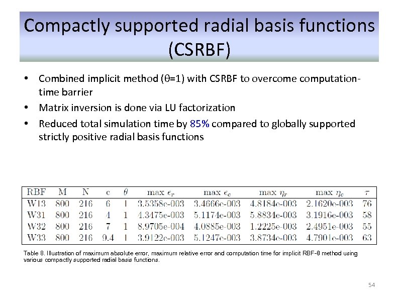 Compactly supported radial basis functions (CSRBF) • Combined implicit method (θ=1) with CSRBF to overcome computationtime barrier • Matrix inversion is done via LU factorization • Reduced total simulation time by 85% compared to globally supported strictly positive radial basis functions Table 8. Illustration of maximum absolute error, maximum relative error and computation time for implicit RBF-θ method using various compactly supported radial basis functions. 54
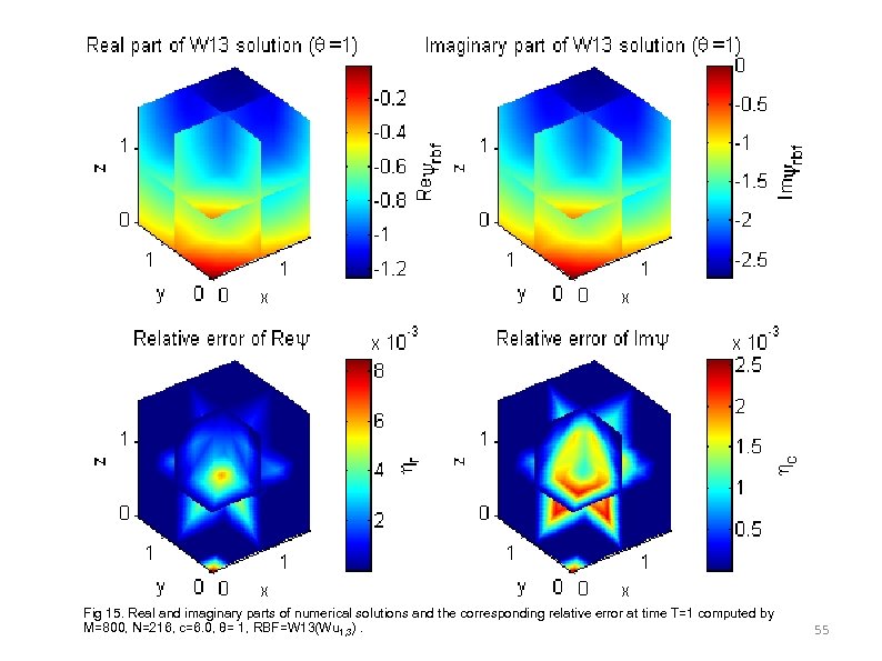 Fig 15. Real and imaginary parts of numerical solutions and the corresponding relative error at time T=1 computed by M=800, N=216, c=6. 0, θ= 1, RBF=W 13(Wu 1, 3). 55
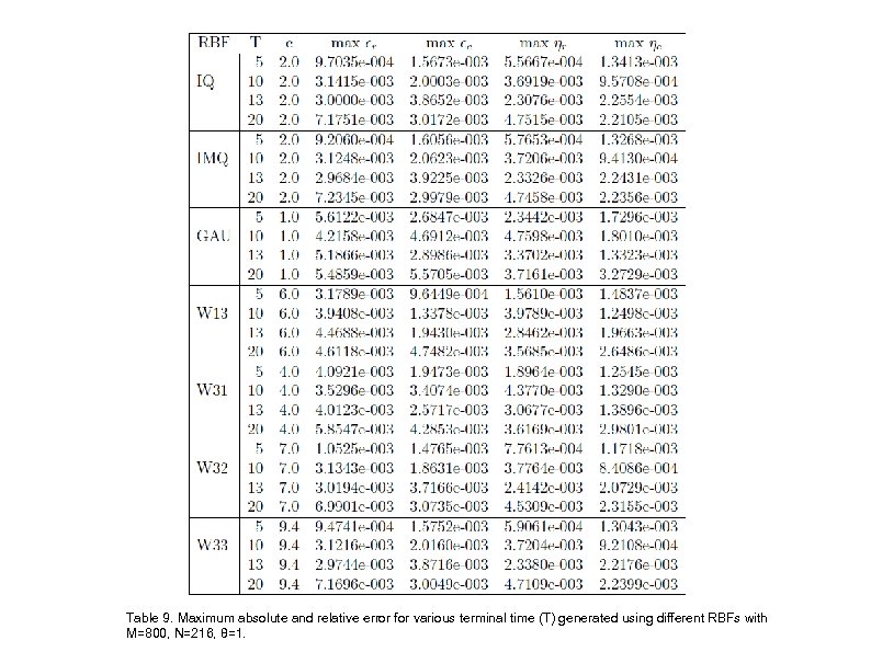 Table 9. Maximum absolute and relative error for various terminal time (T) generated using different RBFs with M=800, N=216, θ=1.
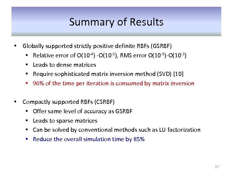 Summary of Results • Globally supported strictly positive definite RBFs (GSRBF) • Relative error of O(10 -4) -O(10 -3), RMS error O(10 -5)-O(10 -3) • Leads to dense matrices • Require sophisticated matrix inversion method (SVD) [10] • 96% of the time per iteration is consumed by matrix inversion • Compactly supported RBFs (CSRBF) • Offer same level of accuracy as GSRBF • Leads to sparse matrices • Can be solved by conventional methods such as LU factorization • Reduce the overall simulation time by 85% 57
 Future Work • Shape parameter selection strategy • More sophisticated time integration scheme – For time dependent external potentials (Nistazakis et al) • On computational enhancements – Utilize more efficient data structures for large scale simulations – Explore parallelism using GPUs or High Performance Computing 58
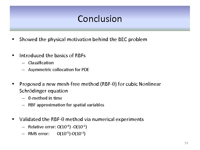 Conclusion • Showed the physical motivation behind the BEC problem • Introduced the basics of RBFs – Classification – Asymmetric collocation for PDE • Proposed a new mesh-free method (RBF-θ) for cubic Nonlinear Schrödinger equation – θ-method in time – RBF approximation for spatial variables • Validated the RBF-θ method via numerical experiments – Relative error: O(10 -4) -O(10 -3) – RMS error: O(10 -5)-O(10 -3) 59
 Thank you very much 60
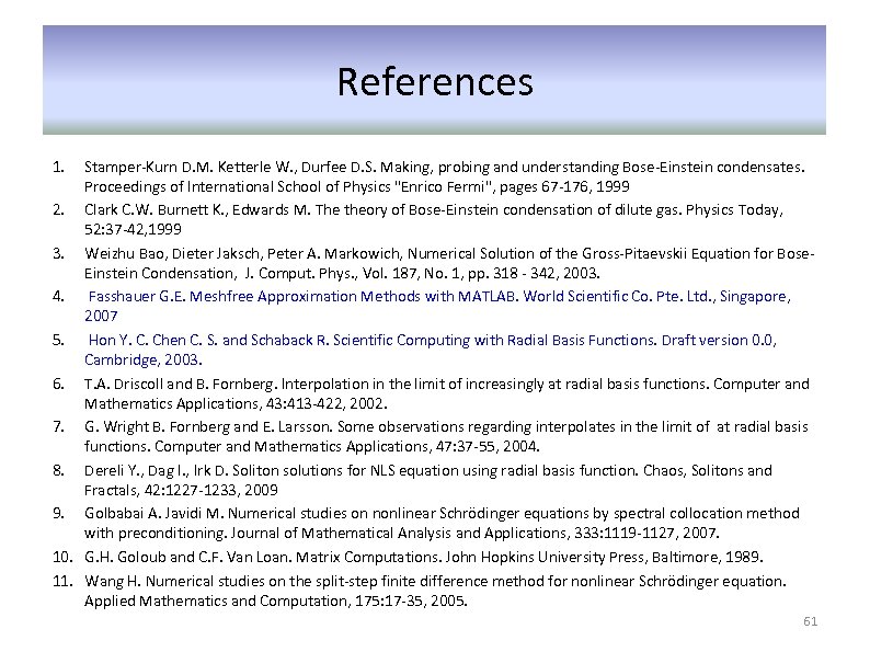 References 1. Stamper-Kurn D. M. Ketterle W. , Durfee D. S. Making, probing and understanding Bose-Einstein condensates. Proceedings of International School of Physics "Enrico Fermi", pages 67 -176, 1999 2. Clark C. W. Burnett K. , Edwards M. The theory of Bose-Einstein condensation of dilute gas. Physics Today, 52: 37 -42, 1999 3. Weizhu Bao, Dieter Jaksch, Peter A. Markowich, Numerical Solution of the Gross-Pitaevskii Equation for Bose. Einstein Condensation, J. Comput. Phys. , Vol. 187, No. 1, pp. 318 - 342, 2003. 4. Fasshauer G. E. Meshfree Approximation Methods with MATLAB. World Scientific Co. Pte. Ltd. , Singapore, 2007 5. Hon Y. C. Chen C. S. and Schaback R. Scientific Computing with Radial Basis Functions. Draft version 0. 0, Cambridge, 2003. 6. T. A. Driscoll and B. Fornberg. Interpolation in the limit of increasingly at radial basis functions. Computer and Mathematics Applications, 43: 413 -422, 2002. 7. G. Wright B. Fornberg and E. Larsson. Some observations regarding interpolates in the limit of at radial basis functions. Computer and Mathematics Applications, 47: 37 -55, 2004. 8. Dereli Y. , Dag I. , Irk D. Soliton solutions for NLS equation using radial basis function. Chaos, Solitons and Fractals, 42: 1227 -1233, 2009 9. Golbabai A. Javidi M. Numerical studies on nonlinear Schrödinger equations by spectral collocation method with preconditioning. Journal of Mathematical Analysis and Applications, 333: 1119 -1127, 2007. 10. G. H. Goloub and C. F. Van Loan. Matrix Computations. John Hopkins University Press, Baltimore, 1989. 11. Wang H. Numerical studies on the split-step finite difference method for nonlinear Schrödinger equation. Applied Mathematics and Computation, 175: 17 -35, 2005. 61


