A Market Impact Model that Works Dan di

A Market Impact Model that Works Dan di. Bartolomeo and Howard Hoffman Northfield Information Services, Inc. CARISMA Seminar June 2007

Main Points for Today u Of the inputs needed to optimally rebalance a portfolio, market impact of large trades is the least researched u Rational boundary conditions need to be incorporated into the empirical estimation of market impact models u We have developed a market impact model that has excellent in-sample explanatory power in several major equity markets, over a database of more than 1. 5 million trades

Motivation u Northfield client comment in 1997: – “Your optimizer just told me to buy five million shares of Ford. From who? ” u Clearly, we want to incorporate market impact into portfolio optimization processes u We would also like to incorporate good market impact estimates into “trade scheduling” that balances reducing market impact against opportunity costs and risk

Total Trading Costs u Most people see trading costs as having several components – – Agency costs Bid/Asked Spread Market Impact (my trade moves the price) Other people’s trades move the price, maybe in my favor. Traders call this “trend cost”. We call it risk u Often overlooked ingredients – My large concurrent trades (my trade in Ford impacts the price of GM) – The implicit opportunity cost of waiting. Unless we’re passive, we want to buy stocks before they go up, not after. If we’re selling we want to sell before they go down, not after

Let’s See What We Can Reasonably Estimate u u u Agency Costs are essentially known in advance Bid/Asked Spreads: Some time variation but reasonably stable Market Impact: Lots of models exist. Underlying factors are highly significant, but explanatory power is typically quite low Trend Costs: They can move the price for or against us. Ex-post is often the largest part of the costs. Pretty darn random. Or so it seems. Market impact and trend costs are hard to disentangle so maybe the market impact models work better than we think

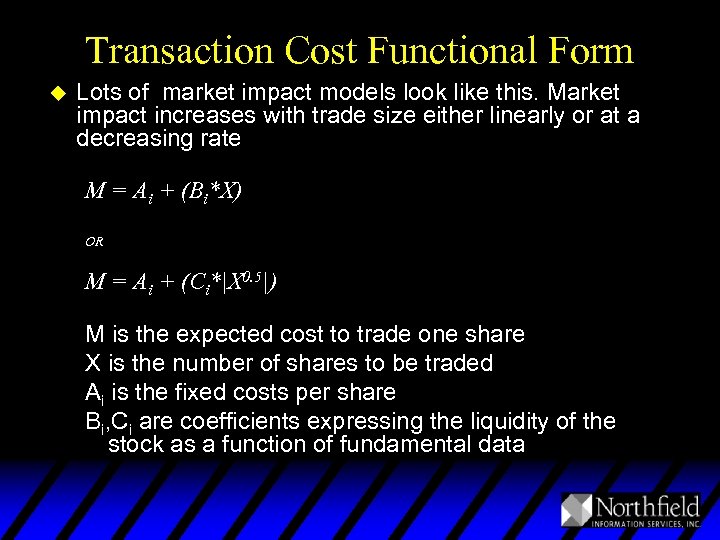Transaction Cost Functional Form u Lots of market impact models look like this. Market impact increases with trade size either linearly or at a decreasing rate M = Ai + (Bi*X) OR M = Ai + (Ci*|X 0. 5|) M is the expected cost to trade one share X is the number of shares to be traded Ai is the fixed costs per share Bi, Ci are coefficients expressing the liquidity of the stock as a function of fundamental data

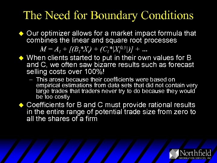The Need for Boundary Conditions u u Our optimizer allows for a market impact formula that combines the linear and square root processes M = Ai + [(Bi*Xt) + (Ci*|Xt 0. 5|)] + … When clients started to put in their own values for B and C, we often saw bizarre results such as forecast selling costs over 100%! – This arose because their coefficients were based on empirical estimations from data sets that did not contain very large trades that traders never try to do because they would be too costly u Coefficients for B and C must provide rational results in the entire range of potential trade size from zero to all the shares of a firm

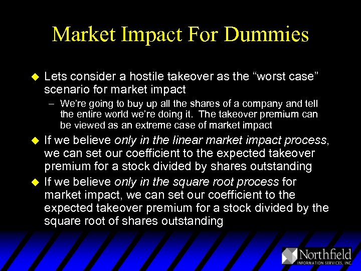Market Impact For Dummies u Lets consider a hostile takeover as the “worst case” scenario for market impact – We’re going to buy up all the shares of a company and tell the entire world we’re doing it. The takeover premium can be viewed as an extreme case of market impact u u If we believe only in the linear market impact process, we can set our coefficient to the expected takeover premium for a stock divided by shares outstanding If we believe only in the square root process for market impact, we can set our coefficient to the expected takeover premium for a stock divided by the square root of shares outstanding

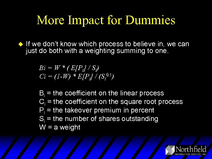More Impact for Dummies u If we don’t know which process to believe in, we can just do both with a weighting summing to one. Bi = W * ( E[Pi] / Si) Ci = (1 -W) * E[Pi] / (Si 0. 5) Bi = the coefficient on the linear process Ci = the coefficient on the square root process Pi = the takeover premium in percent Si = the number of shares outstanding W = a weight

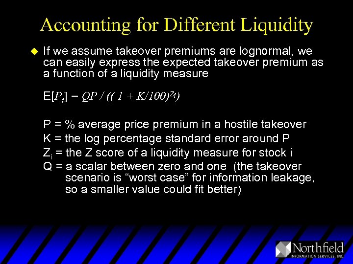Accounting for Different Liquidity u If we assume takeover premiums are lognormal, we can easily express the expected takeover premium as a function of a liquidity measure E[Pi] = QP / (( 1 + K/100)Zi) P = % average price premium in a hostile takeover K = the log percentage standard error around P Zi = the Z score of a liquidity measure for stock i Q = a scalar between zero and one (the takeover scenario is “worst case” for information leakage, so a smaller value could fit better)

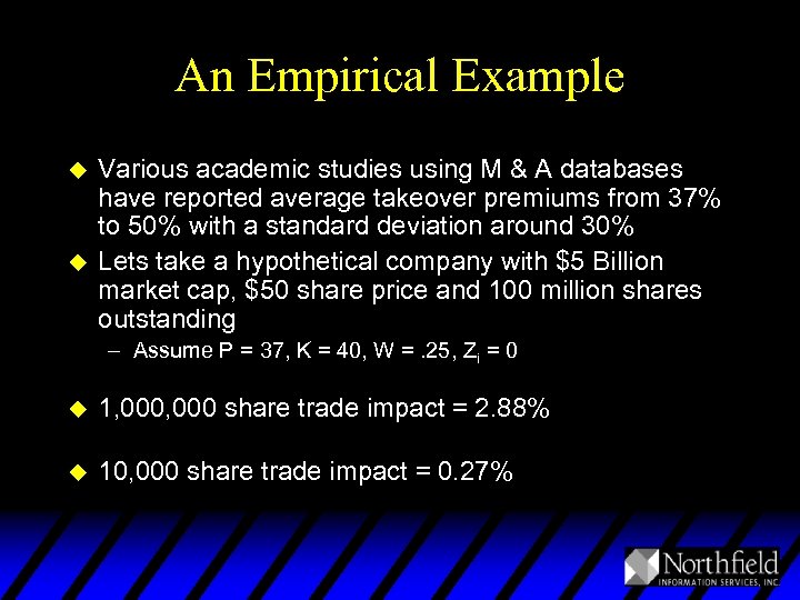An Empirical Example u u Various academic studies using M & A databases have reported average takeover premiums from 37% to 50% with a standard deviation around 30% Lets take a hypothetical company with $5 Billion market cap, $50 share price and 100 million shares outstanding – Assume P = 37, K = 40, W =. 25, Zi = 0 u 1, 000 share trade impact = 2. 88% u 10, 000 share trade impact = 0. 27%

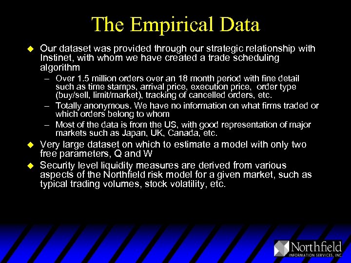The Empirical Data u Our dataset was provided through our strategic relationship with Instinet, with whom we have created a trade scheduling algorithm – Over 1. 5 million orders over an 18 month period with fine detail such as time stamps, arrival price, execution price, order type (buy/sell, limit/market), tracking of cancelled orders, etc. – Totally anonymous. We have no information on what firms traded or which orders belong to whom – Most of the data is from the US, with good representation of major markets such as Japan, UK, Canada, etc. u u Very large dataset on which to estimate a model with only two free parameters, Q and W Security level liquidity measures are derived from various aspects of the Northfield risk model for a given market, such as typical trading volumes, stock volatility, etc.

Measuring Market Impact? u One way to measure market impact would be to compare the price we got on our trade versus the price on the previous trade as a measure of how much our trade “moved the price” – This may not be relevant to us. We care about how much the price moved from the price it was at when we decided to trade the stock u We use an “arrival price” measure. It’s the percentage in price between the execution price and the price that existed in the market when we got the order to transact the stock – Implementation Shortfall described in Perold (1988) – Very noisy relationships since a limit order can sit for hours between arrival and execution. Prices can move around a lot during that time from other people’s trades, not ours

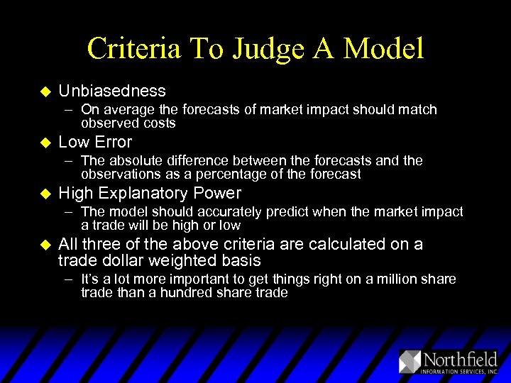Criteria To Judge A Model u Unbiasedness – On average the forecasts of market impact should match observed costs u Low Error – The absolute difference between the forecasts and the observations as a percentage of the forecast u High Explanatory Power – The model should accurately predict when the market impact a trade will be high or low u All three of the above criteria are calculated on a trade dollar weighted basis – It’s a lot more important to get things right on a million share trade than a hundred share trade

An Estimation Subtlety u Using “arrival price cost” as the measure, its possible that the realized market impact of a trade could be negative or zero – We’re buying a stock and the price went down before our order was executed u u However, the forecast market impact is always positive, so we calculate percentage of error with the forecast in the denominator This means that a low percentage of error and a high R-squared are not exactly congruent measures – There is more room to be wrong on one side than the other

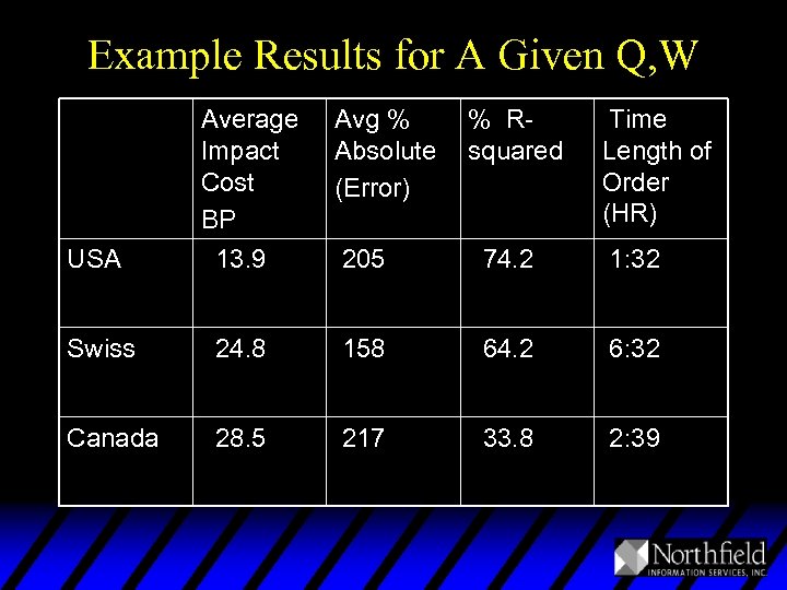Example Results for A Given Q, W Average Impact Cost BP Avg % Absolute (Error) % Rsquared Time Length of Order (HR) USA 13. 9 205 74. 2 1: 32 Swiss 24. 8 158 64. 2 6: 32 Canada 28. 5 217 33. 8 2: 39

Empirical Results Discussion u We are able to isolate values of Q, W that are economically reasonable and fit the data extremely well in several countries (US, Canada, Switzerland) based on our current choice of liquidity measures u The same liquidity measures fit poorly in other countries such as the UK and Japan. More research is needed u We will continue this line of research until we cover all stocks in our Global Equity Risk Model

In the Portfolio Optimization Context u u u Most people who use an optimizer for rebalancing portfolios use some form of transaction cost estimate Many people use some form of non-linear transaction cost function that includes a market impact component If interdependencies between market impacts are not accounted for, large trades will be incorrectly specified – – Consider two sets of orders Buy 5 Million shares of Ford, Buy 5 Million shares of GM Buy 5 Million shares of Ford, Sell 5 Million shares of GM Are expected market impacts the same?

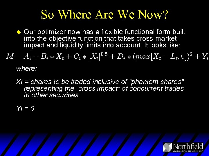So Where Are We Now? u Our optimizer now has a flexible functional form built into the objective function that takes cross-market impact and liquidity limits into account. It looks like: where: Xt = shares to be traded inclusive of “phantom shares” representing the “cross impact” of concurrent trades in other securities Yi = 0

Amortization Functions u In a portfolio optimization process, total estimated costs must be traded off against expected alpha and risk – Amortize trading costs over the expected holding period – Adjust the amortization rate, G, to reflect “the probability of realization” which is less than one for finite holding periods u u For small transaction costs, arithmetic amortization is sufficient, but if costs are large we need to consider compounding Assume a trade with 20% trading cost and an expected holding period of one year. – We can get an expected alpha improvement of 20%. But if we give up 20% of our money now, and invest at 20% for one period, we only end up with 96% of the money we have now.

Optimal Trade Scheduling u If we know the urgency of trades, and the likely impact, we can create optimal trade “schedules” to break up large trades into a series of smaller trades – We still need an assumption about the extent that market impact in one period is a permanent move in the price and how much is transient. u Once we have that, the problem becomes a dynamic optimization. Normally solved using Bellman equation methods – Our formulation uses a nearly traditional optimization with time made endogenous. Think of many stocks all called IBM that each can only be traded in one period: IBM (to trade Monday), IBM (to trade Tuesday), etc. u Our trade scheduling algorithm with Instinet went live a few months ago

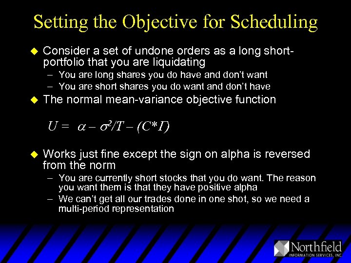Setting the Objective for Scheduling u Consider a set of undone orders as a long shortportfolio that you are liquidating – You are long shares you do have and don’t want – You are short shares you do want and don’t have u The normal mean-variance objective function U = a – s 2/T – (C*G) u Works just fine except the sign on alpha is reversed from the norm – You are currently short stocks that you do want. The reason you want them is that they have positive alpha – We can’t get all our trades done in one shot, so we need a multi-period representation

Permanent and Temporary Market Impact u If our trades in any given stock are far apart in time, price movements caused by our trades will be independent of one another u If our trades follow each other with little time in between, market impact effects will have a cascading effect as each trade moves the price from where the previous trade left it u We call this persistent portion of market impact “stickiness”, and account for it in the solution when the length of our discrete time blocks is short

Why Mean Variance? u Some trading algorithms try minimizing the standard deviation of trading costs – From a process control perspective minimizing the uncertainty (standard deviation) rather than variance seems intuitive u However, the variance in trading costs impact ending portfolio values is half the variance, and is not linearly related to the standard deviation – Consider trading a 100 Yen portfolio with a trading cost of 10% twice. Ending wealth is 81 Yen – Consider two trades with an average of 10% cost, 0% cost and 20% cost. Ending wealth is 80 Yen – The decimal variance of the second case is 0. 01 so the expected loss is 0. 005 per observation. This checks since 0. 005 * 100 * 2 = 1

The Trade Schedule u u u Lets assume we want to finish all our open trades over a two trading day period We can break the two days into discrete time blocks, either by clock time or by “expected share of day’s volume” (e. g. each block is the length of clock time that usually trades 5% of the days volume Think of a spreadsheet where each order is a row and each time block is a column. – We want the matrix of orders such that all orders are completed by the end of the schedule – That maximizes our objectives: capturing short term alpha, minimizing risk and market impact u After each period is experienced, we can check that the expected orders were executed; if not, we can rerun the schedule based on the remaining shares and time periods

Conclusions u Our search for a market impact model that both fits the data well (at least in some markets) and is rationality bounded has been fruitful. u We can incorporate reasonable estimates of market impact for any size trade into both optimization and trade scheduling processes u We expect to incorporate this market impact model into the Instinet trade scheduling system during 2007

References u u u u Wade, Nick. “Northfield Market Impact Model”, July 1998 Cox, Berry. “Implementation Shortfall: Modeling Transaction Costs”, CQA Presentation, April 1998 di. Bartolomeo, Dan. “Optimization with Composite Assets Using Implied Covariance Matrices”. Northfield Working Paper, 1998 Perold, Andre F. "The Implementation Shortfall: Paper Versus Reality, " Journal of Portfolio Management, 1988, v 14(3), 4 -9. Barclay, Michael J. and Jerold B. Warner. "Stealth Trading And Volatility: Which Trades Move Prices? , " Journal of Financial Economics, 1993, v 34(3), 281 -306. Bertsimas, Dimitris and Andrew W. Lo. "Optimal Control Of Execution Costs, " Journal of Financial Markets, 1998, v 1(1, Apr), 1 -50. Bertsimas, Dimitris, Paul Hummel and Andrew Lo. “Optimal Control of Execution Costs for Portfolios”, Computing in Science and Engineering, November 1999

References u u u u Angel, James J. , Gary L. Gastineau and Clifford J. Weber. "Reducing The Market Impact Of Large Stock Trades, " Journal of Portfolio Management, 1997, v 24(1, Fall), 69 -76. Hasbrouck, Joel. "The Dynamics Of Discrete Bid And Ask Quotes, " Journal of Finance, 1999, v 54(6, Dec), 2109 -2142. Roll, Richard. "A Simple Implicit Measure Of The Effective Bid. Ask Spread In An Efficient Market, " Journal of Finance, 1984, v 39(4), 1127 -1139. Ho, Thomas S. Y. , Robert A. Schwartz and David K. Whitcomb. "The Trading Decision And Market Clearing Under Transaction Price Uncertainty, " Journal of Finance, 1985, v 40(1), 21 -42. Almgren, Robert and Neil Chriss. “Optimal Execution of Portfolio Transactions”, Journal of Risk, 2001, v 3, 5 -39 Almgren, Robert and Neil Chriss, “Optimal Execution with Non. Linear Impact Costs and Trading Enhanced Risk”. Working Paper 2001 Malamut, Roberto. “Multi-Period Optimization Techniques for Trade Scheduling”, QWAFAFEW New York, April 2002

References u u u Walkling, Ralph A. "Predicting Tender Offer Success: A Logistic Analysis, " Journal of Financial and Quantitative Analysis, 1985, v 20(4), 461 -478. Billett, Matthew T. and Mike Ryngaert. "Capital Structure, Asset Structure And Equity Takeover Premiums In Cash Tender Offers, " Journal of Corporate Finance, 1997, v 3(2, Apr), 141 -165. Eckbo, B. Espen and Herwig Langohr. "Information Disclosure, Method Of Payment, And Takeover Premiums: Public And Private Tender Offers In France, " Journal of Financial Economics, 1989, v 24(2), 363 -404. Walkling, Ralph A. and Robert O. Edmister. "Determinants Of Tender Offer Premiums, " Financial Analyst Journal, 1985, v 41(1), 27, 30 -37. Wansley, James W. , William R. Lane and Salil Sarkar. "Managements' View On Share Repurchase And Tender Offer Premiums, " Financial Management, 1989, v 18(3), 97 -110.