bab7c89f4c479f00542bde0a6d8ef501.ppt
- Количество слайдов: 37
 A Lecture Presentation in Power. Point to accompany Exploring Economics Second Edition by Robert L. Sexton Copyright © 2002 Thomson Learning, Inc. Thomson Learning™ is a trademark used herein under license. ALL RIGHTS RESERVED. Instructors of classes adopting EXPLORING ECONOMICS, Second Edition by Robert L. Sexton as an assigned textbook may reproduce material from this publication for classroom use or in a secure electronic network environment that prevents downloading or reproducing the copyrighted material. Otherwise, no part of this work covered by the copyright hereon may be reproduced or used in any form or by any means—graphic, electronic, or mechanical, including, but not limited to, photocopying, recording, taping, Web distribution, information networks, or information storage and retrieval systems—without the written permission of the publisher. Printed in the United States of America ISBN 0030342333 Copyright © 2002 by Thomson Learning, Inc.
 The Aggregate Expenditures Model Copyright © 2002 by Thomson Learning, Inc.
 Consumption Depends on Disposable Income n Marginal propensity to save (MPS) n the change in savings divided by the change in disposable income Copyright © 2002 by Thomson Learning, Inc.
 Consumption Depends on Disposable Income n Current consumption spending depends on many factors. n n n age family size interest rates expected future disposable income wealth current disposable income n Empirical studies show that most people’s consumption spending is closely tied to their disposable income. Copyright © 2002 by Thomson Learning, Inc.
 Consumption Depends on Disposable Income n If your disposable income is n n n $0, you spend $8, 000 (that means you have to borrow or reduce your existing savings just to survive). $20, 000, you’ll spend $8, 000 plus 75 percent of $20, 000 (which equals $15, 000), for total spending of $23, 000. $40, 000, you’ll spend $8, 000 plus 75 percent of $40, 000 (which equals $30, 000), for total spending of $38, 000. Copyright © 2002 by Thomson Learning, Inc.
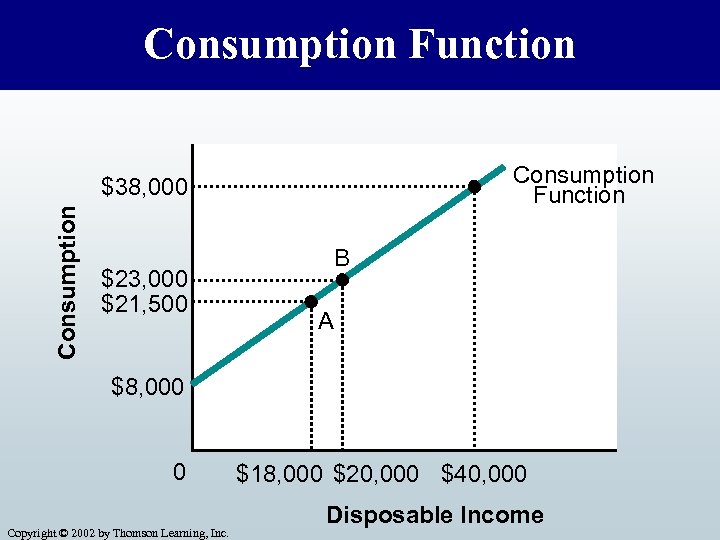 Consumption Function Consumption $38, 000 $23, 000 $21, 500 B A $8, 000 0 Copyright © 2002 by Thomson Learning, Inc. $18, 000 $20, 000 $40, 000 Disposable Income
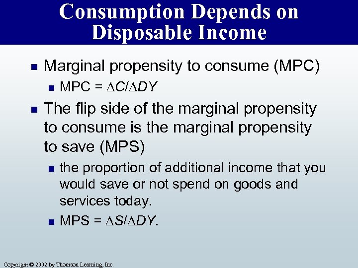 Consumption Depends on Disposable Income n Marginal propensity to consume (MPC) n n MPC = C/ DY The flip side of the marginal propensity to consume is the marginal propensity to save (MPS) n n the proportion of additional income that you would save or not spend on goods and services today. MPS = S/ DY. Copyright © 2002 by Thomson Learning, Inc.
 Consumption Depends on Disposable Income n n The slope of the line represents the marginal propensity to consume. Aggregate consumption gives a functional relationship called a consumption function. Copyright © 2002 by Thomson Learning, Inc.
 Consumption Depends on Disposable Income n Let’s suppose consumption spending in the economy is something like $1 trillion plus 75 percent of income. n n Consumption is partly autonomous (the $1 trillion part, which people would spend no matter what their income, which depends on the current interest rate, real wealth, debt, and expectations), and partly induced, which means it depends on income, the portion that’s equal to 75 percent of income. Copyright © 2002 by Thomson Learning, Inc.
 Consumption Depends on Disposable Income n If we assume that investment, government purchases, and net exports are zero, aggregate expenditure is just equal to the amount of consumption spending represented by our consumption function. Copyright © 2002 by Thomson Learning, Inc.
 Equilibrium in the Aggregate Expenditure Model n At the equilibrium level of output, planned production of goods and services (RGDP) is equal to the aggregate expenditures (AE)—the total planned spending for these goods and services. Copyright © 2002 by Thomson Learning, Inc.
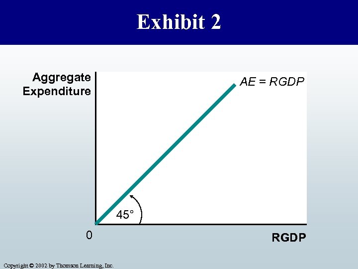 Exhibit 2 Aggregate Expenditure AE = RGDP 45° 0 Copyright © 2002 by Thomson Learning, Inc. RGDP
 Equilibrium in the Aggregate Expenditure Model n The 45 -degree line illustrates coordinates where the number on the horizontal axis, representing the amount of output in the economy, is equal to the number on the vertical axis, representing the amount of aggregate expenditure in the economy. n If equilibrium output is $5 trillion, then aggregate expenditure must equal $5 trillion. Copyright © 2002 by Thomson Learning, Inc.
 Equilibrium in the Aggregate Expenditure Model n What if output were lower than its equilibrium level RGDP 1? Copyright © 2002 by Thomson Learning, Inc.
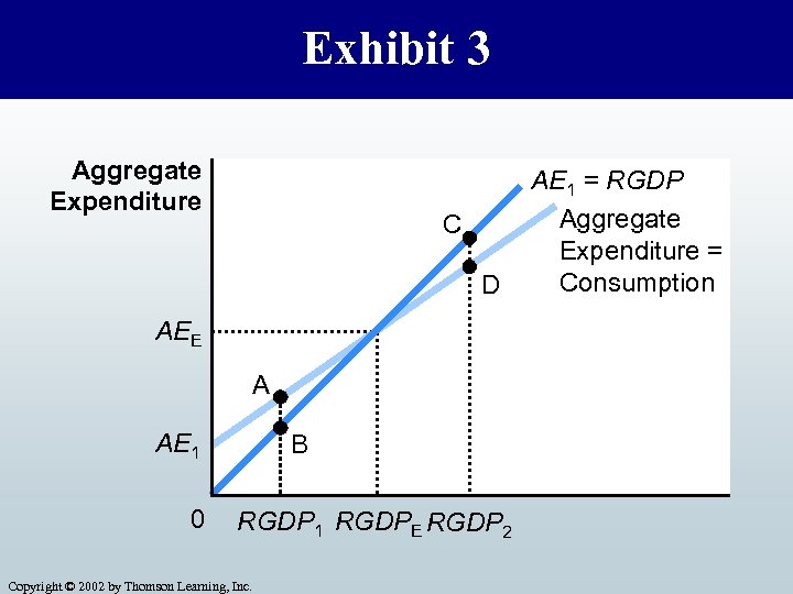 Exhibit 3 Aggregate Expenditure C D AEE A AE 1 0 B RGDP 1 RGDPE RGDP 2 Copyright © 2002 by Thomson Learning, Inc. AE 1 = RGDP Aggregate Expenditure = Consumption
 Equilibrium in the Aggregate Expenditure Model n When output is RGDP 1, AE is greater than output labeled the distance AB n n n People would be buying more goods and services (A) than were being produced (B). Inventories would decrease. Production would increase to increase inventory stocks. Output would increase in the economy. This process would continue until output reached its equilibrium level, where the two lines intersect. Copyright © 2002 by Thomson Learning, Inc.
 Equilibrium in the Aggregate Expenditure Model n When output is RGDP 2, above equilibrium, economic forces would act to reduce output. n n n AE (D) is less than output (C). People wouldn’t buy all the output. Production would be reduced. Inventories would be bulging. Rational firms would reduce output and production until inventory stocks return to the desired level and the equilibrium level of output was reached. Copyright © 2002 by Thomson Learning, Inc.
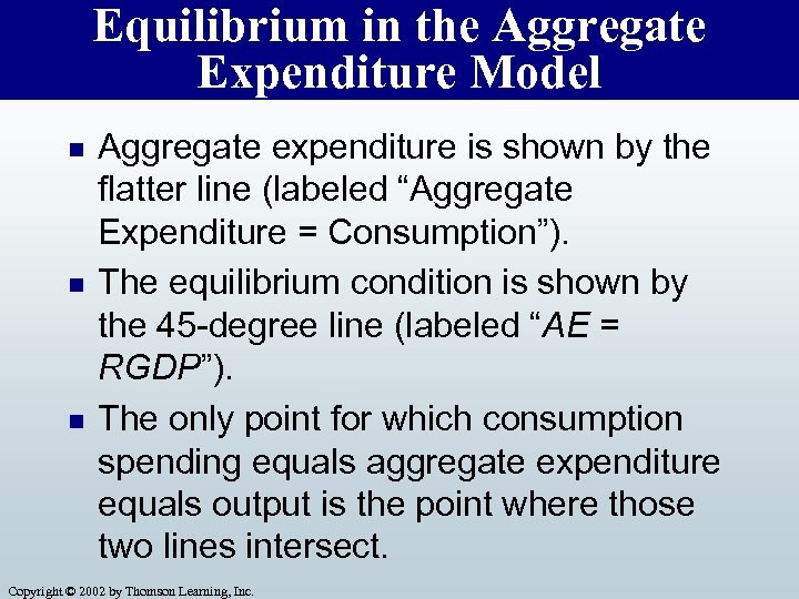 Equilibrium in the Aggregate Expenditure Model n n n Aggregate expenditure is shown by the flatter line (labeled “Aggregate Expenditure = Consumption”). The equilibrium condition is shown by the 45 -degree line (labeled “AE = RGDP”). The only point for which consumption spending equals aggregate expenditure equals output is the point where those two lines intersect. Copyright © 2002 by Thomson Learning, Inc.
 Adding Investment, Government Purchases, and Net Exports n n Suppose that consumption depends on the level of income or output in the economy, but that investment, government purchases, and net exports do not. Instead, investment, government purchases, and net exports depend on other factors in the economy such as interest rates, political considerations, or the condition of foreign economies. Copyright © 2002 by Thomson Learning, Inc.
 Adding Investment, Government Purchases, and Net Exports n Now, aggregate expenditure (AE) consists of n n n consumption (C) plus investment (I) plus government purchases (G) plus net exports (NX): AE C + I + G + NX. Copyright © 2002 by Thomson Learning, Inc.
 Adding Investment, Government Purchases, and Net Exports n n The components of aggregate expenditure result in an upward-sloping line because consumption increases as income increases. Allowing for investment, government purchases, and net exports, the autonomous portion of aggregate expenditure is larger. Copyright © 2002 by Thomson Learning, Inc.
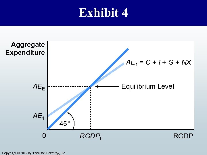 Exhibit 4 Aggregate Expenditure AE 1 = C + I + G + NX Equilibrium Level AEE AE 1 45° 0 Copyright © 2002 by Thomson Learning, Inc. RGDPE RGDP
 Adding Investment, Government Purchases, and Net Exports n As before, the equilibrium occurs where the two lines cross, that is, where the aggregate expenditure line intersects the equilibrium line, which is the 45 degree line. Copyright © 2002 by Thomson Learning, Inc.
 Shifts in Aggregate Expenditure n Aggregate expenditure increases due to n n n More optimistic expectations Easier credit conditions (interest rates decline) Real wealth increases Firms increase their investment (especially if their productivity rises or the interest rate declines) Government increases its spending Net exports rise as foreign economies improve their economic health Copyright © 2002 by Thomson Learning, Inc.
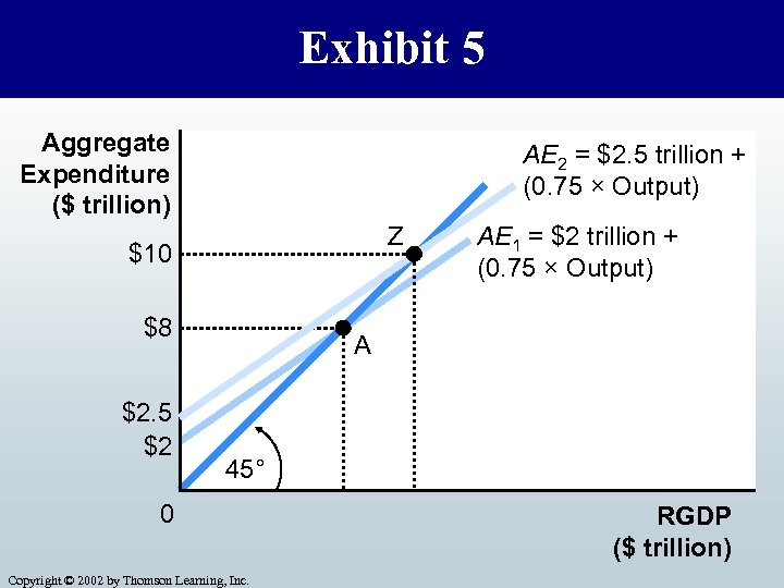 Exhibit 5 Aggregate Expenditure ($ trillion) AE 2 = $2. 5 trillion + (0. 75 × Output) Z $10 $8 $2. 5 $2 AE 1 = $2 trillion + (0. 75 × Output) A 45° 0 Copyright © 2002 by Thomson Learning, Inc. RGDP ($ trillion)
 From Aggregate Expenditure to Aggregate Demand n n To go from the aggregate expenditure model to aggregate demand, all we need to consider is how the price level affects the components of aggregate demand. Now we allow the components of aggregate expenditure to depend on the price level. Copyright © 2002 by Thomson Learning, Inc.
 From Aggregate Expenditure to Aggregate Demand n When the price level falls n n n Consumption rises, because people’s real wealth rises (the real wealth effect). Investment increases because interest rates decline (the interest-rate effect). Furthermore, net exports rise because domestic goods become relatively cheaper than foreign goods (the open economy effect). Copyright © 2002 by Thomson Learning, Inc.
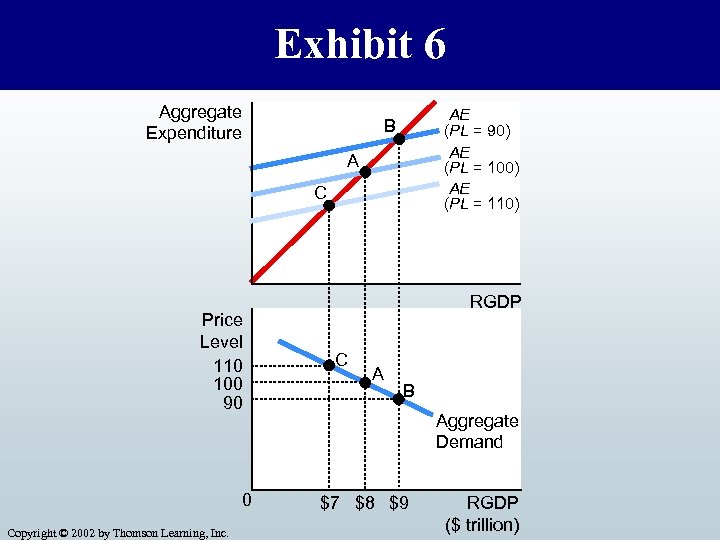 Exhibit 6 Aggregate Expenditure AE (PL = 90) AE (PL = 100) AE (PL = 110) B A C Price Level 110 100 90 0 Copyright © 2002 by Thomson Learning, Inc. RGDP C A B Aggregate Demand $7 $8 $9 RGDP ($ trillion)
 From Aggregate Expenditure to Aggregate Demand n When the price level is 100, n n n the aggregate expenditure is the curve labeled AE(PL = 100) in the top diagram. The equilibrium in the Keynesian-cross model occurs at point A. Point A in the bottom diagram corresponds to a price level of 100 and output of $8 trillion. Copyright © 2002 by Thomson Learning, Inc.
 From Aggregate Expenditure to Aggregate Demand n If the price level falls from 100 to 90, n n n The aggregate-expenditure curve shifts up to AE(PL = 90). A new equilibrium occurs at point B. Point B in the bottom diagram corresponds to price level 90 and output $9 trillion. Copyright © 2002 by Thomson Learning, Inc.
 From Aggregate Expenditure to Aggregate Demand n If the price level rises to 110, n n n The aggregate-expenditure curve shifts down to AE(PL = 110). The new equilibrium in the aggregate expenditure diagram occurs at point C. Point C in the bottom diagram corresponds to a price level of 110 and output of $7 trillion. Copyright © 2002 by Thomson Learning, Inc.
 From Aggregate Expenditure to Aggregate Demand n n The higher the price level, the lower is aggregate demand. Carrying out this same experiment for every possible price level would trace out the entire aggregate demand curve, as shown. Copyright © 2002 by Thomson Learning, Inc.
 Shifts in Aggregate Demand n Changes in any of the components of aggregate expenditure that occur for any reason other than a change in the price level or output lead to a shift of the aggregate demand curve. n n whenever the autonomous parts of consumption, investment, government purchases, or net exports increase Such a change would shift the aggregate-expenditure curve upwards. Copyright © 2002 by Thomson Learning, Inc.
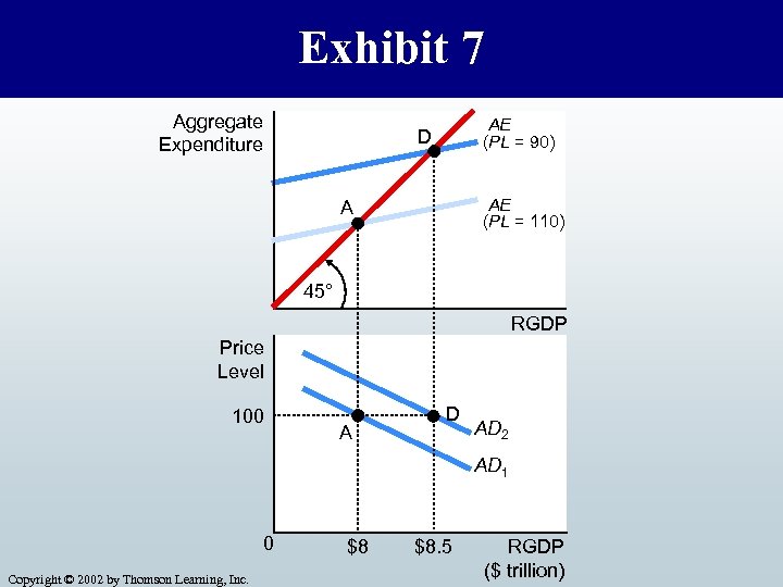 Exhibit 7 Aggregate Expenditure AE (PL = 90) D AE (PL = 110) A 45° RGDP Price Level 100 A D AD 2 AD 1 0 Copyright © 2002 by Thomson Learning, Inc. $8 $8. 5 RGDP ($ trillion)
 Shifts in Aggregate Demand n n We denote the original aggregateexpenditure curve AE 1 and the new aggregate-expenditure curve AE 2. Originally the economy is in equilibrium at point A with output of $8 trillion and a price level of 100. Copyright © 2002 by Thomson Learning, Inc.
 Shifts in Aggregate Demand n n After the increase in government purchases, the aggregate-expenditure curve shifts up, moving the economy to a new equilibrium at point D with output of $8. 5 trillion and price level remaining at 100. For any other given price level, equilibrium output would also be higher after an increase in government purchases. Copyright © 2002 by Thomson Learning, Inc.
 Shifts in Aggregate Demand n So, the new aggregate demand curve on the lower diagram shifts to the right. Copyright © 2002 by Thomson Learning, Inc.


