A Fiscal Policy The Keynesian View of

A. Fiscal Policy

The Keynesian View of Fiscal Policy n n Keynesian theory highlights the potential of fiscal policy as a tool capable of reducing fluctuations in demand. When an economy is operating below its potential output, the Keynesian model suggests that the government should institute expansionary fiscal policy -- it should either: n n increase the government’s purchases of goods & services, and/or, cut taxes.

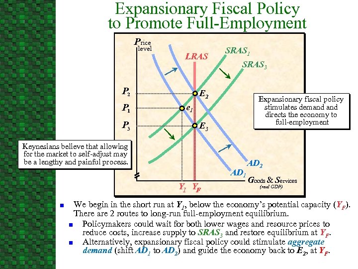Expansionary Fiscal Policy to Promote Full-Employment Price level LRAS P 2 P 1 P 3 SRAS 1 SRAS 3 E 2 Expansionary fiscal policy stimulates demand directs the economy to full-employment e 1 E 3 Keynesians believe that allowing for the market to self-adjust may be a lengthy and painful process. AD 1 YF n AD 2 Goods & Services (real GDP) We begin in the short run at Y 1, below the economy’s potential capacity (YF). There are 2 routes to long-run full-employment equilibrium. n Policymakers could wait for both lower wages and resource prices to reduce costs, increase supply to SRAS 3 and restore equilibrium at YF. n Alternatively, expansionary fiscal policy could stimulate aggregate demand (shift AD 1 to AD 2) and guide the economy back to E 2, at YF.

The Keynesian View of Fiscal Policy n n When inflation is a potential problem, the Keynesian analysis suggests a shift toward a more restrictive fiscal policy: n reduce government spending, and/or, n raise taxes. Keynesians challenged the view that the government’s should always be balance its budget. n Rather than balancing the budget annually, Keynesians argued that counter-cyclical policy should be used to offset fluctuations in aggregate demand.

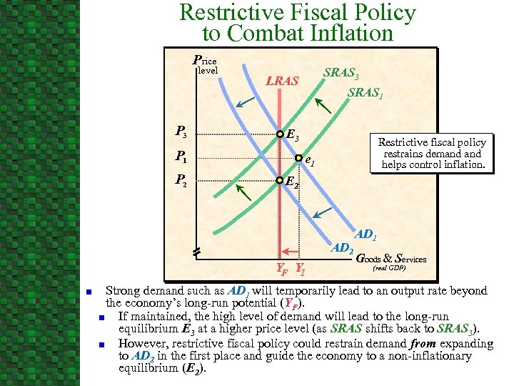Restrictive Fiscal Policy to Combat Inflation Price level P 3 SRAS 1 E 3 P 1 P 2 SRAS 3 LRAS Restrictive fiscal policy restrains demand helps control inflation. e 1 E 2 AD 2 YF Y 1 n AD 1 Goods & Services (real GDP) Strong demand such as AD 1 will temporarily lead to an output rate beyond the economy’s long-run potential (YF). n If maintained, the high level of demand will lead to the long-run equilibrium E 3 at a higher price level (as SRAS shifts back to SRAS 3). n However, restrictive fiscal policy could restrain demand from expanding to AD 2 in the first place and guide the economy to a non-inflationary equilibrium (E 2).

Fiscal Policy and the Crowding-out Effect n The Crowding-out Effect: -- indicates that the increased borrowing to finance a budget deficit will push real interest rates up and thereby retard private spending, reducing the stimulus effect of expansionary fiscal policy. n The implications of the crowding-out analysis are symmetrical. n n Restrictive fiscal policy will reduce real interest rates and "crowd in" private spending. Crowding-out Effect in an open economy: -- Larger budget deficits and higher real interest rates also lead to an inflow of capital, appreciation in the dollar, and a decline in net exports.

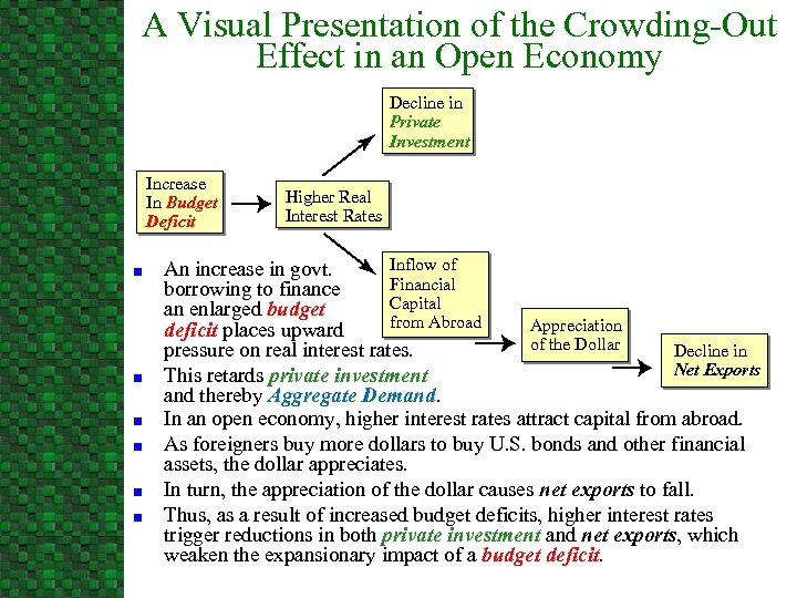A Visual Presentation of the Crowding-Out Effect in an Open Economy Decline in Private Investment Increase In Budget Deficit n n n Higher Real Interest Rates Inflow of An increase in govt. Financial borrowing to finance Capital an enlarged budget from Abroad Appreciation deficit places upward of the Dollar pressure on real interest rates. Decline in Net Exports This retards private investment and thereby Aggregate Demand. In an open economy, higher interest rates attract capital from abroad. As foreigners buy more dollars to buy U. S. bonds and other financial assets, the dollar appreciates. In turn, the appreciation of the dollar causes net exports to fall. Thus, as a result of increased budget deficits, higher interest rates trigger reductions in both private investment and net exports, which weaken the expansionary impact of a budget deficit.

The New Classical View of Fiscal Policy n The New classical view stresses that: u u n debt financing merely substitutes higher future taxes for lower current taxes, and thus, budget deficits affect the timing of taxes, but not their magnitude. New Classics argue that when debt is substituted for taxes u u people will save the increased income so they will be able to pay the higher future taxes, thus, the budget deficit does not stimulate aggregate demand.

The New Classical View of Fiscal Policy n n Similarly, the real interest rate is unaffected by deficits since people will save more in order to pay the higher future taxes. According to the new classical view, fiscal policy is completely impotent. It does not effect output, employment, or real interest rates.

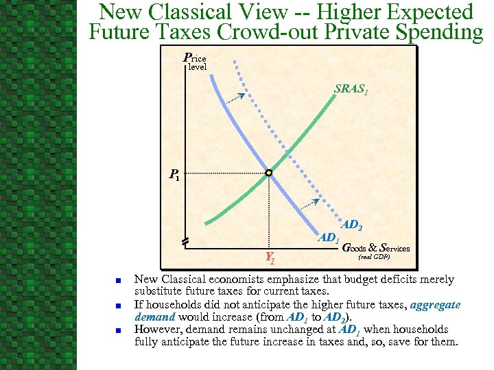New Classical View -- Higher Expected Future Taxes Crowd-out Private Spending Price level SRAS 1 P 1 AD 1 Y 1 n n n AD 2 Goods & Services (real GDP) New Classical economists emphasize that budget deficits merely substitute future taxes for current taxes. If households did not anticipate the higher future taxes, aggregate demand would increase (from AD 1 to AD 2). However, demand remains unchanged at AD 1 when households fully anticipate the future increase in taxes and, so, save for them.

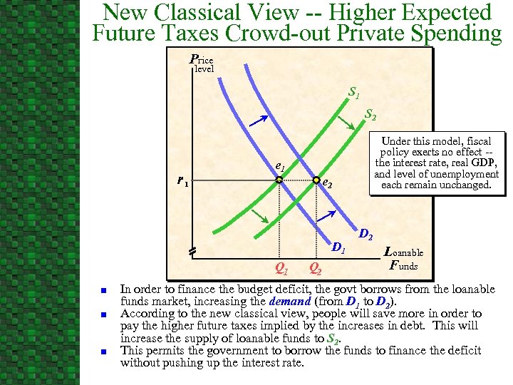New Classical View -- Higher Expected Future Taxes Crowd-out Private Spending Price level S 1 S 2 r 1 e 2 D 1 Q 1 n n n Under this model, fiscal policy exerts no effect -the interest rate, real GDP, and level of unemployment each remain unchanged. Q 2 D 2 Loanable Funds In order to finance the budget deficit, the govt borrows from the loanable funds market, increasing the demand (from D 1 to D 2). According to the new classical view, people will save more in order to pay the higher future taxes implied by the increases in debt. This will increase the supply of loanable funds to S 2. This permits the government to borrow the funds to finance the deficit without pushing up the interest rate.

Fiscal Policy: -- Problems with Proper Timing n n Various time lags make proper timing of changes in discretionary fiscal policy difficult. Discretionary fiscal policy is like a two-edged sword; it can both harm and help. u u If timed correctly, it may reduce economic instability. If timed incorrectly, however, it may increase economic instability.

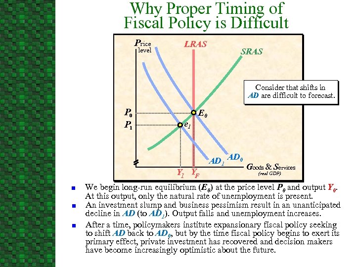Why Proper Timing of Fiscal Policy is Difficult Price level LRAS SRAS Consider that shifts in AD are difficult to forecast. P 0 P 1 e 1 E 0 Y 1 YF n n n AD 1 AD 0 Goods & Services (real GDP) We begin long-run equilibrium (E 0) at the price level P 0 and output Y 0. At this output, only the natural rate of unemployment is present. An investment slump and business pessimism result in an unanticipated decline in AD (to AD 1). Output falls and unemployment increases. After a time, policymakers institute expansionary fiscal policy seeking to shift AD back to AD 0, but by the time fiscal policy begins to exert its primary effect, private investment has recovered and decision makers have become increasingly optimistic about the future.

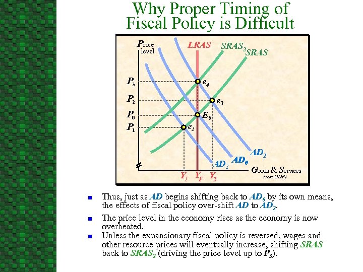Why Proper Timing of Fiscal Policy is Difficult Price level LRAS P 3 e 4 P 2 P 0 P 1 SRAS 2 SRAS e 2 e 1 E 0 AD 2 AD 0 AD 1 Goods & Services Y 1 YF Y 2 (real GDP) n n n Thus, just as AD begins shifting back to AD 0 by its own means, the effects of fiscal policy over-shift AD to AD 2. The price level in the economy rises as the economy is now overheated. Unless the expansionary fiscal policy is reversed, wages and other resource prices will eventually increase, shifting SRAS back to SRAS 2 (driving the price level up to P 3).

Fiscal Policy: -- Problems with Proper Timing n Automatic Stabilizers: -- without any new legislative action, they tend to increase the budget deficit (or reduce the surplus) during a recession and increase the surplus (or reduce the deficit) during an economic boom. n Examples of Automatic Stabilizers: u u u Unemployment Compensation Corporate Profit Tax A Progressive Income Tax

Fiscal Policy as a Tool: -- A Modern Synthesis n n n The proper timing of discretionary fiscal policy is both difficult to achieve and of crucial importance. Automatic stabilizers reduce the fluctuation of aggregate demand help to direct the economy toward full-employment. Fiscal policy is much less potent than the early Keynesian view implied.

Supply-side Effects of Fiscal Policy n From a supply-side viewpoint, the marginal tax rate is of crucial importance: u n A reduction in marginal tax rates increases the reward derived from added work, investment, saving, and other activities that become less heavily taxed. High marginal tax rates will tend to retard total output because they will: u u u Discourage work effort and reduce the productive efficiency of labor, Adversely affect the rate of capital formation and the efficiency of its use, and, Encourage individuals to substitute less desired tax-deductible goods for more desired nondeductible goods.

Supply-side Effects of Fiscal Policy n n Thus, changes in marginal tax rates, particularly high marginal rates, may exert an impact on aggregate supply because the changes will influence the relative attractiveness of productive activity in comparison to leisure and tax avoidance. Impact of supply-side effects u u u Are likely to take place over a lengthy time period. There is some evidence that countries with high taxes grow more slowly—France and Germany versus United Kingdom. While the significance of supply-side effects are controversial, there is evidence they are important for taxpayers facing extremely high rate, say rates of 40 percent and above.

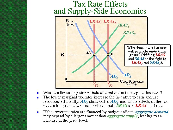Tax Rate Effects and Supply-Side Economics Price level LRAS 1 LRAS 2 SRAS 1 SRAS 2 P 0 E 1 E 2 AD 1 YF 1 n n n YF 2 With time, lower tax rates will promote more rapid growth (shifting LRAS and SRAS to the right to LRAS 2 and SRAS 2). AD 2 Goods & Services (real GDP) What are the supply-side effects of a reduction in marginal tax rates? The lower marginal tax rates increase the incentive to earn and use resources efficiently. AD 1 shifts out to AD 2, and as the effects of the tax cut are long-run as well as short-run, both SRAS and LRAS shift out. If the lower tax rates are financed by budget deficits, aggregate demand may expand by a larger amount than aggregate supply, leading to an increase in the price level.

B. Money and the Banking System

What Is Money? n A Medium of Exchange n A Store of Value n A Unit of Account -- An asset that is used to buy and sell goods & services. -- An asset that will allow people to transfer purchasing power from one period to another. -- The units of measurement used by people to post prices and keep track of revenues and costs.

The Supply of Money n The components of the M 1 money supply are: u u Currency Checking Deposits (including demand deposits and interest-earning checking deposits) u n Traveler's checks The M 2 money supply is a broader measure that includes: u u M 1, Savings, Time deposits, and, Money mutual funds.

The Business of Banking n The banking industry includes: u u u n n n Banks accept deposits and use part of them to extend loans and make investments. Banks are profit-seeking institutions. Banks play a central role in the capital (loanable funds) market: u n savings and loans, credit unions, and, commercial banks. They help to bring together people who want to save for the future with those who want to borrow in order to undertake investment projects. The banking system is a fractional reserve system: -- Banks maintain only a fraction of their assets in reserves to meet the requirements of depositors.

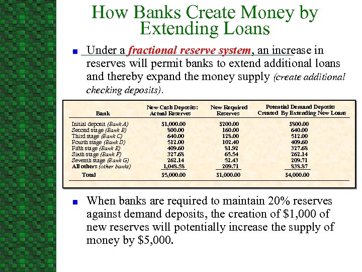How Banks Create Money by Extending Loans n Under a fractional reserve system, an increase in reserves will permit banks to extend additional loans and thereby expand the money supply (create additional checking deposits). Bank New Cash Deposits: Actual Reserves New Required Reserves Initial deposit (Bank A) Second stage (Bank B) Third stage (Bank C) Fourth stage (Bank D) Fifth stage (Bank E) Sixth stage (Bank F) Seventh stage (Bank G) All others (other banks) Total $1, 000. 00 800. 00 640. 00 512. 00 409. 60 327. 68 262. 14 1, 048. 58 $5, 000. 00 $200. 00 160. 00 128. 00 102. 40 81. 92 65. 54 52. 43 209. 71 $1, 000. 00 n Potential Demand Deposits Created By Extending New Loans $800. 00 640. 00 512. 00 409. 60 327. 68 262. 14 209. 71 838. 87 $4, 000. 00 When banks are required to maintain 20% reserves against demand deposits, the creation of $1, 000 of new reserves will potentially increase the supply of money by $5, 000.

How Banks Create Money by Extending Loans n n n The lower the percentage of the reserve requirement, the greater is the potential expansion in the money supply resulting from the creation of new reserves. The fractional reserve requirement places a ceiling on potential money creation from new reserves. The actual deposit multiplier will be less than the potential because: u u Some persons will hold currency rather than bank deposits. Some banks may not use all their excess reserves to extend loans.

The Three Tools the Fed Uses to Control the Money Supply n Reserve requirements: -- a % of a specified liability category (for example transaction accounts) that banking institutions are required to hold as reserves against that type of liability. u u When the Fed lowers the required reserve ratio, it creates excess reserves and allows banks to extend additional loans, expanding the money supply. Raising the reserve requirements has the opposite effect.

The Three Tools the Fed Uses to Control the Money Supply n Open Market Operations: -- the buying and selling of U. S. Government securities (national debt in the form of bonds) by the Fed. u u This is the primary tool used by Fed. When the Fed buys bonds the money supply will expand, because: u the bond buyers will acquire money, and, u bank reserves will increase, placing banks in a position to expand the money supply through the extension of additional loans. u When the Fed sells bonds the money supply will contract because: u bond buyers are giving up money in exchange for securities, and, u the reserves available to banks will decline, causing them to extend fewer loans.

The Three Tools the Fed Uses to Control the Money Supply n Discount Rate: -- the interest rate the Fed charges banking institutions for borrowed funds. u u An increase in the discount rate is restrictive (decreases the money supply) because it discourages banks from borrowing from the Federal Reserve to extend new loans. A reduction in the discount rate is expansionary (increases the money supply) because it makes borrowing from the Federal Reserve less costly.

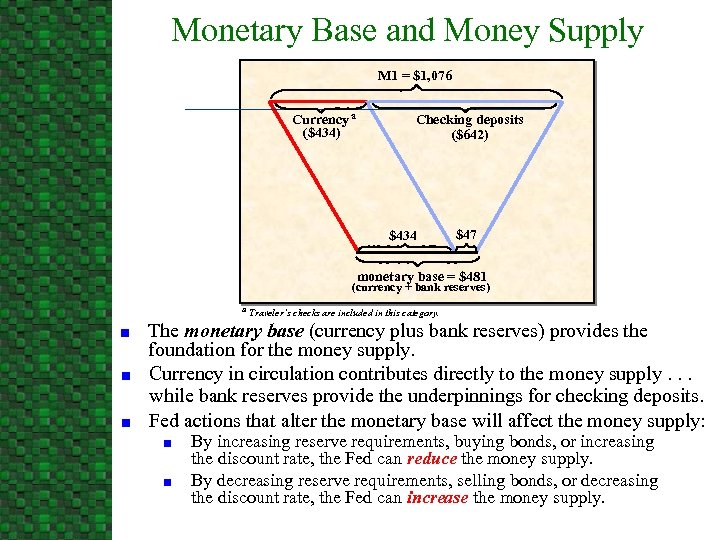Monetary Base and Money Supply M 1 = $1, 076 Currency a ($434) Checking deposits ($642) $434 $47 monetary base = $481 (currency + bank reserves) a Traveler’s checks are included in this category. n n n The monetary base (currency plus bank reserves) provides the foundation for the money supply. Currency in circulation contributes directly to the money supply. . . while bank reserves provide the underpinnings for checking deposits. Fed actions that alter the monetary base will affect the money supply: n n By increasing reserve requirements, buying bonds, or increasing the discount rate, the Fed can reduce the money supply. By decreasing reserve requirements, selling bonds, or decreasing the discount rate, the Fed can increase the money supply.

Ambiguities in the Meaning and Measurement of the Money Supply n Interest earning checking deposits u u n Less costly to hold than currency and demand deposits. Their introduction in the early 1980’s changed the nature of the M 1 money supply. Widespread use of the U. S. dollar outside of the United States u u More than one-half and perhaps as much as two-thirds of U. S. currency is held overseas. This reduces the reliability of the M 1 money supply measure.

Ambiguities in the Meaning and Measurement of the Money Supply n n Sweeping of various interest-earning checking accounts into Money Market Deposit Accounts The increasing availability of low-fee stock and bond mutual funds Debit Cards and Electronic Money Summary: u u Recent financial innovations and other structural changes have blurred the meaning of money and reduced the reliability of the various money supply measures. In the Computer-Age, continued change in this area is likely.

C. Monetary Policy

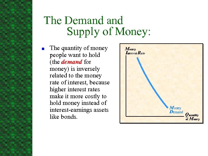The Demand Supply of Money: n The quantity of money people want to hold (the demand for money) is inversely related to the money rate of interest, because higher interest rates make it more costly to hold money instead of interest-earnings assets like bonds. Money Interest Rate Money Demand Quantity of Money

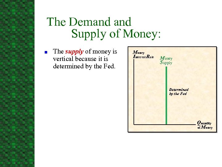The Demand Supply of Money: n The supply of money is vertical because it is determined by the Fed. Money Interest Rate Money Supply Determined by the Fed Quantity of Money

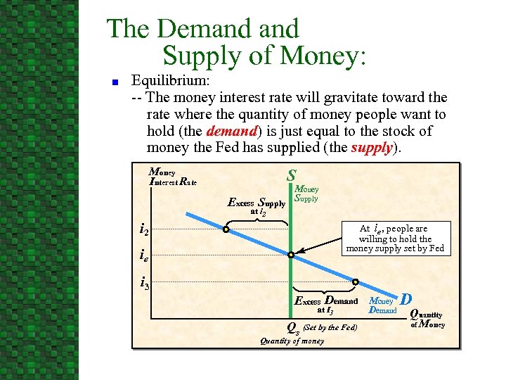The Demand Supply of Money: n Equilibrium: -- The money interest rate will gravitate toward the rate where the quantity of money people want to hold (the demand) is just equal to the stock of money the Fed has supplied (the supply). Money Interest Rate S Excess Supply Money Supply at i 2 At ie , people are willing to hold the money supply set by Fed i 2 ie i 3 Excess Demand Money at I 3 Qs (Set by the Fed) Quantity of money Demand D Quantity of Money

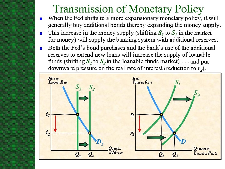Transmission of Monetary Policy n n n When the Fed shifts to a more expansionary monetary policy, it will generally buy additional bonds thereby expanding the money supply. This increase in the money supply (shifting S 1 to S 2 in the market for money) will supply the banking system with additional reserves. Both the Fed’s bond purchases and the bank’s use of the additional reserves to extend new loans will increase the supply of loanable funds (shifting S 1 to S 2 in the loanable funds market). . . and put downward pressure on the real rate of interest (reduction to r 2). Money Interest Rate S 1 Real Interest Rate S 2 S 1 S 2 i 1 r 1 i 2 r 2 D 1 Qs Qb D Quantity of Money Q 1 Q 2 Quantity of Loanable Funds

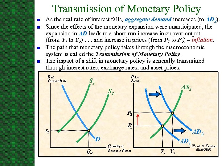Transmission of Monetary Policy n n As the real rate of interest falls, aggregate demand increases (to AD 2). Since the effects of the monetary expansion were unanticipated, the expansion in AD leads to a short-run increase in current output (from Y 1 to Y 2). . . and increase in prices (from P 1 to P 2) – inflation. The path that monetary policy takes through the macroeconomic system is called the Transmission of Monetary Policy. The impact of a shift in monetary policy is generally transmitted through interest rates, exchange rates, and asset prices. Real Interest Rate Price Level S 1 AS 1 S 2 P 1 r 2 AD 2 D Q 2 Quantity of Loanable Funds AD 1 Y 2 Goods & Services (Real GDP)

A Shift to a More Expansionary Monetary Policy n n During expansionary monetary policy the Fed may buy bonds, reduce the discount rate, or reduce the reserve requirements for deposits. The Fed generally buys bonds, which: n n increases bond prices, and, creates additional bank reserves, while it, places downward pressure on real interest rates. As a result, an unanticipated shift to a more expansionary policy will stimulate aggregate demand thereby increase both output and employment.

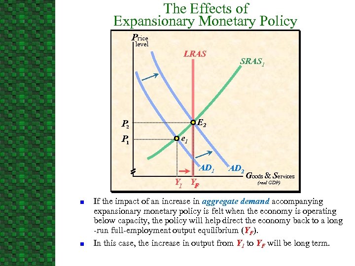The Effects of Expansionary Monetary Policy Price level LRAS E 2 P 1 e 1 AD 1 YF n n SRAS 1 AD 2 Goods & Services (real GDP) If the impact of an increase in aggregate demand accompanying expansionary monetary policy is felt when the economy is operating below capacity, the policy will help direct the economy back to a long -run full-employment output equilibrium (YF). In this case, the increase in output from Y 1 to YF will be long term.

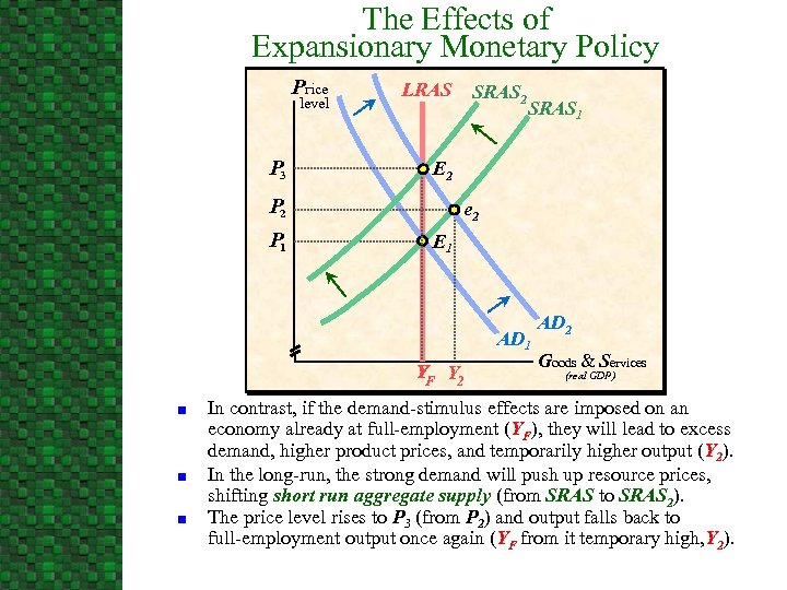The Effects of Expansionary Monetary Policy Price level P 3 LRAS SRAS 1 E 2 P 1 SRAS 2 e 2 E 1 AD 1 YF Y 2 n n n AD 2 Goods & Services (real GDP) In contrast, if the demand-stimulus effects are imposed on an economy already at full-employment (YF), they will lead to excess demand, higher product prices, and temporarily higher output (Y 2). In the long-run, the strong demand will push up resource prices, shifting short run aggregate supply (from SRAS to SRAS 2). The price level rises to P 3 (from P 2) and output falls back to full-employment output once again (YF from it temporary high, Y 2).

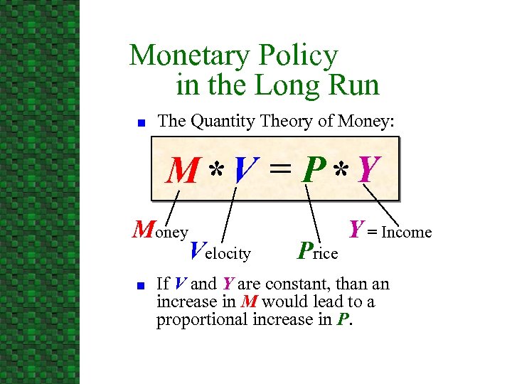Monetary Policy in the Long Run n The Quantity Theory of Money: M * V = P *Y Money Velocity n Price Y = Income If V and Y are constant, than an increase in M would lead to a proportional increase in P.

Monetary Policy in the Long Run n The Long-Run Implications of Modern Analysis: u u u In the long run, the primary impact will be on prices rather than on real output. When expansionary monetary policy leads to rising prices, decision makers eventually anticipate the higher inflation rate and build it into their choices. As this happens, money interest rates, wages, and incomes will reflect the expectation of inflation, and so real interest rates, wages, and output will return to their long-run normal levels.

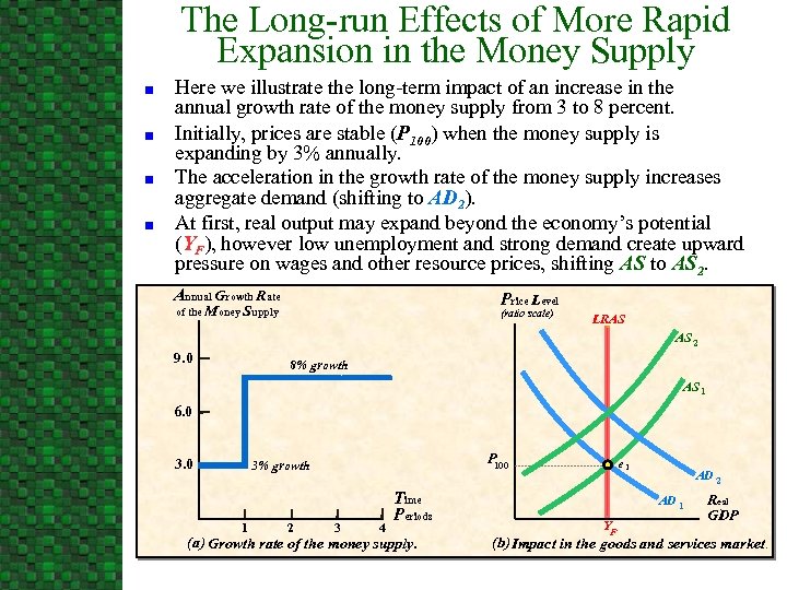The Long-run Effects of More Rapid Expansion in the Money Supply n n Here we illustrate the long-term impact of an increase in the annual growth rate of the money supply from 3 to 8 percent. Initially, prices are stable (P 100) when the money supply is expanding by 3% annually. The acceleration in the growth rate of the money supply increases aggregate demand (shifting to AD 2). At first, real output may expand beyond the economy’s potential (YF), however low unemployment and strong demand create upward pressure on wages and other resource prices, shifting AS to AS 2. Annual Growth Rate Price Level of the Money Supply (ratio scale) LRAS AS 2 9. 0 8% growth AS 1 6. 0 3. 0 P 100 3% growth 1 2 3 4 Time Periods (a) Growth rate of the money supply. e 1 AD 2 AD 1 YF Real GDP (b) Impact in the goods and services market.

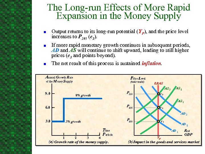The Long-run Effects of More Rapid Expansion in the Money Supply Output returns to its long-run potential (YF), and the price level increases to P 105 (e 2). n If more rapid monetary growth continues in subsequent periods, AD and AS will continue to shift upward, leading to still higher prices (e 3 and points beyond). The net result of this process is sustained inflation. n n Annual Growth Rate Price Level of the Money Supply 9. 0 (ratio scale) P 110 8% growth LRAS AS 3 AS 2 e 3 AS 1 P 105 6. 0 e 2 AD 3 3. 0 P 100 3% growth 1 2 3 4 Time Periods (a) Growth rate of the money supply. e 1 AD 2 AD 1 YF Real GDP (b) Impact in the goods and services market.

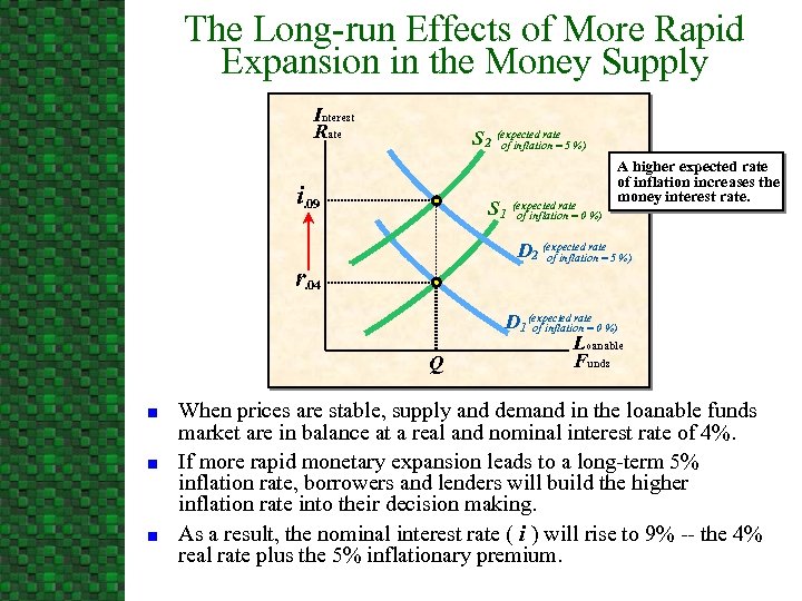The Long-run Effects of More Rapid Expansion in the Money Supply Interest Rate S 2 (expected rate 5 %) of inflation = i. 09 S 1 (expected rate 0 %) of inflation = D 2 (expected rate 5 %) of inflation = r. 04 Q n n n A higher expected rate of inflation increases the money interest rate. D 1 (expected rate 0 %) of inflation = Loanable Funds When prices are stable, supply and demand in the loanable funds market are in balance at a real and nominal interest rate of 4%. If more rapid monetary expansion leads to a long-term 5% inflation rate, borrowers and lenders will build the higher inflation rate into their decision making. As a result, the nominal interest rate ( i ) will rise to 9% -- the 4% real rate plus the 5% inflationary premium.

Monetary Policy When Effects Are Anticipated n n When the effects of policy are anticipated prior to their occurrence, the short‑run impact of an increase in the money supply is similar to its impact in the long run. Nominal prices and interest rates rise, but real output remains unchanged.

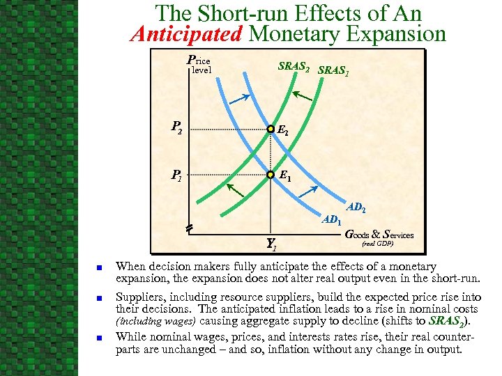The Short-run Effects of An Anticipated Monetary Expansion Price SRAS 2 SRAS 1 level P 2 E 2 P 1 E 1 AD 1 Y 1 n n n AD 2 Goods & Services (real GDP) When decision makers fully anticipate the effects of a monetary expansion, the expansion does not alter real output even in the short-run. Suppliers, including resource suppliers, build the expected price rise into their decisions. The anticipated inflation leads to a rise in nominal costs (including wages) causing aggregate supply to decline (shifts to SRAS 2). While nominal wages, prices, and interests rates rise, their real counterparts are unchanged – and so, inflation without any change in output.

Interest Rates and Monetary Policy n n While the Fed can strongly influence shortterm interest rates, its impact on long-term rates is much more limited. Interest rates can be a misleading indicator of monetary policy: u u In the long run, expansionary monetary policy leads to inflation and high interest rates, rather than low interest rates. Similarly, restrictive monetary policy, when pursued over a lengthy time period, leads to low inflation and low interest rates.

The Effects of Monetary Policy: -- A Summary n n n An unanticipated shift to a more expansionary (restrictive) monetary policy will temporarily stimulate (retard) output and employment. The stabilizing effects of a change in monetary policy are dependent upon the state of the economy when the effects of the policy change are observed. Persistent growth of the money supply at a rapid rate will cause inflation. Money interest rates and the inflation rate will be directly related. There will be only a loose year-to-year relationship between shifts in monetary policy and changes in output and prices.

D. Stabilization Policy, Output and Employment

Promoting Economic Stability -- Activist and Non-activist Views n Goals of Stabilization Policy: u u u n A stable growth of real GDP, A relatively stable level of prices, A high level of employment (low unemployment). Activists' Views of Stabilization Policy: u u u The self corrective mechanism works slowly if at all, Policy-makers will be able to alter macro-policy, injecting stimulus to help pull the economy out of recession and implementing restraint to help control inflation, According to the activist s view, policy-makers are more likely to keep the economy on track when they are free to apply stimulus or restraint based on forecasting devices and current economic indicators.

Promoting Economic Stability -- Activist and Non-activist Views n Non-activists' Views of Stabilization Policy: u u u The self-corrective mechanism of markets works pretty well, Greater stability would result if stable, predictable policies based on predetermined rules were followed, Non-activists argue that the problems of proper timing and political considerations undermine the effectiveness of discretionary macro policy as a stabilization tool.

Practical Problems With Discretionary Macro Policy n Lags and the Problem of Timing: u u n After a change in policy has been undertaken, there will be a time lag before it exerts a major impact. This means policy makers need to forecast economic conditions several months in the future in order to institute policy changes effectively. Politics and Timing of Policy Changes: u Policy changes may be driven by political considerations rather than stabilization.

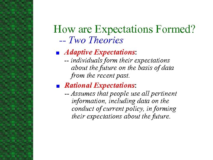How are Expectations Formed? -- Two Theories n Adaptive Expectations: -- individuals form their expectations about the future on the basis of data from the recent past. n Rational Expectations: -- Assumes that people use all pertinent information, including data on the conduct of current policy, in forming their expectations about the future.

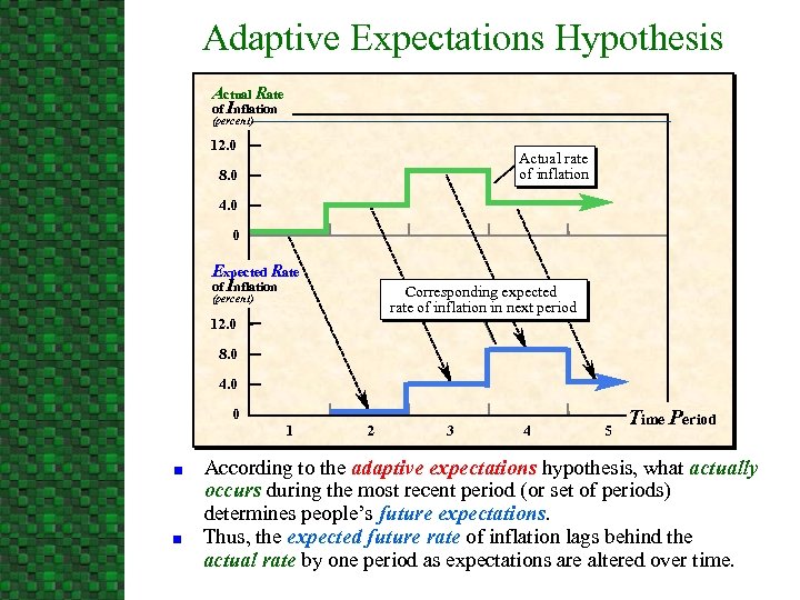Adaptive Expectations Hypothesis Actual Rate of Inflation (percent) 12. 0 Actual rate of inflation 8. 0 4. 0 0 Expected Rate of Inflation Corresponding expected rate of inflation in next period (percent) 12. 0 8. 0 4. 0 0 n n 1 2 3 4 5 Time Period According to the adaptive expectations hypothesis, what actually occurs during the most recent period (or set of periods) determines people’s future expectations. Thus, the expected future rate of inflation lags behind the actual rate by one period as expectations are altered over time.

How Macro Policy Works – The Implications of Adaptive and Rational Expectations n n n With adaptive expectations, an unanticipated shift to a more expansionary policy will temporarily stimulate output and employment. With rational expectations, expansionary policy will not generate a systematic change in output. Both expectations theories indicate that sustained expansionary policies will lead to inflation without permanently increasing output and employment.

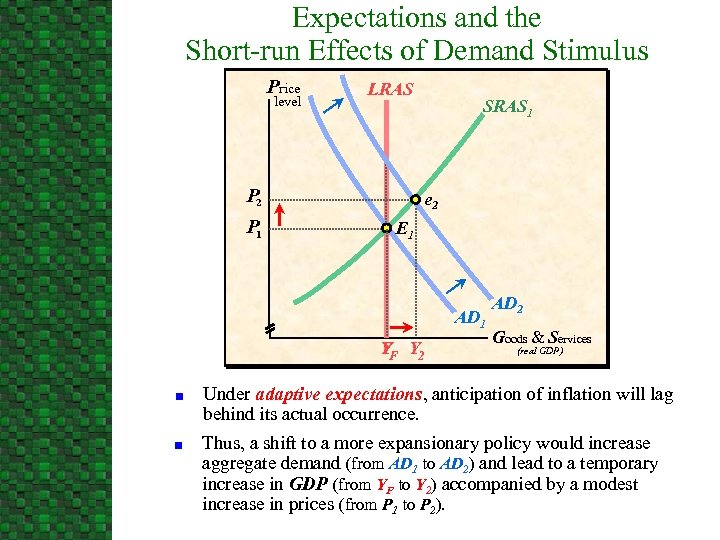Expectations and the Short-run Effects of Demand Stimulus Price level LRAS P 2 P 1 SRAS 1 e 2 E 1 AD 1 YF Y 2 n n AD 2 Goods & Services (real GDP) Under adaptive expectations, anticipation of inflation will lag behind its actual occurrence. Thus, a shift to a more expansionary policy would increase aggregate demand (from AD 1 to AD 2) and lead to a temporary increase in GDP (from YF to Y 2) accompanied by a modest increase in prices (from P 1 to P 2).

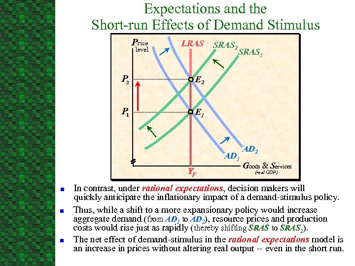Expectations and the Short-run Effects of Demand Stimulus Price level LRAS P 2 SRAS 1 E 2 P 1 SRAS 2 E 1 AD 1 YF n n n AD 2 Goods & Services (real GDP) In contrast, under rational expectations, decision makers will quickly anticipate the inflationary impact of a demand-stimulus policy. Thus, while a shift to a more expansionary policy would increase aggregate demand (from AD 1 to AD 2), resource prices and production costs would rise just as rapidly (thereby shifting SRAS to SRAS 2). The net effect of demand-stimulus in the rational expectations model is an increase in prices without altering real output -- even in the short run.

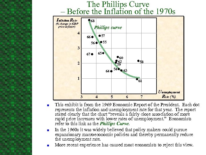The Phillips Curve – Before the Inflation of the 1970 s Inflation Rate 68 (% change in GDP price deflator) Phillips curve 4 57 66 55 56 3 65 67 60 62 59 54 63 2 64 1 61 3 n n n 58 4 5 6 7 Unemployment Rate (%) This exhibit is from the 1969 Economic Report of the President. Each dot represents the inflation and unemployment rate for that year. The report stated clearly that the chart “reveals a fairly close association of more rapid price increases with lower rates of unemployment. ” Economists refer to this link as the Phillips Curve. In the 1960 s it was widely believed that policy makers could pursue expansionary macroeconomic policies and thereby permanently reduce the unemployment rate. More recent experience has caused most economists to reject this view.

Early Views About the Phillips Curve n n n During the 1960 s, most economists thought there was an inverse relationship between inflation and unemployment. This led to the belief that even though expansionary policies would lead to some inflation, they would also result in a long-lasting lower rate of unemployment. Stability of the inflation-unemployment relationship proved to be an illusion. u u As the inflation rate rose from 3% in the late 1960 s to double-digit levels during 1974 -1975, the rate of unemployment rose from less than 4% to more than 8%. As high rates of inflation continued in the latter half of the 1970 s, so too did the high rates of unemployment.

Early Views About the Phillips Curve n The error of early Phillips Curve proponents: -- Failure to consider expectations u u u Integration of expectations into the Phillips curve analysis indicates that any trade-off between inflation and unemployment will be short-lived. An unanticipated shift to a more expansionary policy may temporarily reduce the unemployment rate, but when decision makers come to anticipate the higher rate of inflation, unemployment will return to its natural rate. Even high rates of inflation will fail to reduce unemployment once they are anticipated by decision makers.

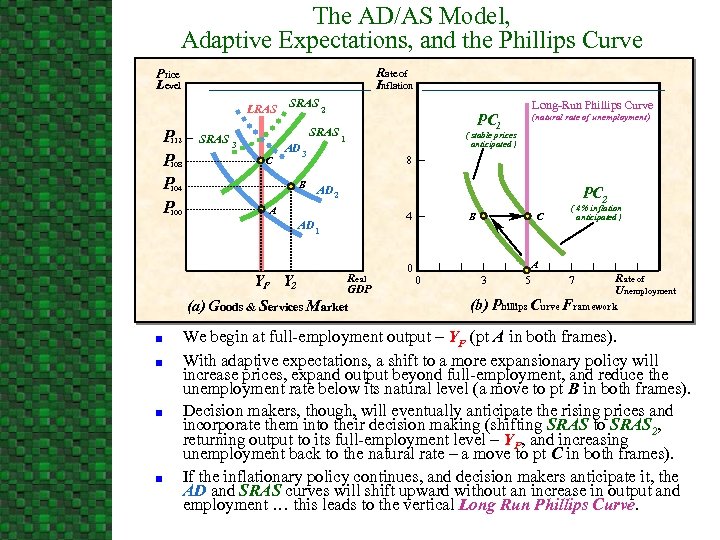The AD/AS Model, Adaptive Expectations, and the Phillips Curve Rate of Inflation Price Level LRAS P 112 P 108 P 104 P 100 SRAS 3 C SRAS 2 AD 3 B n n ( stable prices anticipated ) AD 2 Real GDP (a) Goods & Services Market n (natural rate of unemployment) 8 AD 1 n PC 1 SRAS 1 A YF Y 2 Long-Run Phillips Curve PC 2 4 0 B C ( 4% inflation anticipated ) A 0 3 5 7 Rate of Unemployment (b) Phillips Curve Framework We begin at full-employment output – YF (pt A in both frames). With adaptive expectations, a shift to a more expansionary policy will increase prices, expand output beyond full-employment, and reduce the unemployment rate below its natural level (a move to pt B in both frames). Decision makers, though, will eventually anticipate the rising prices and incorporate them into their decision making (shifting SRAS to SRAS 2, returning output to its full-employment level – YF, and increasing unemployment back to the natural rate – a move to pt C in both frames). If the inflationary policy continues, and decision makers anticipate it, the AD and SRAS curves will shift upward without an increase in output and employment … this leads to the vertical Long Run Phillips Curve.

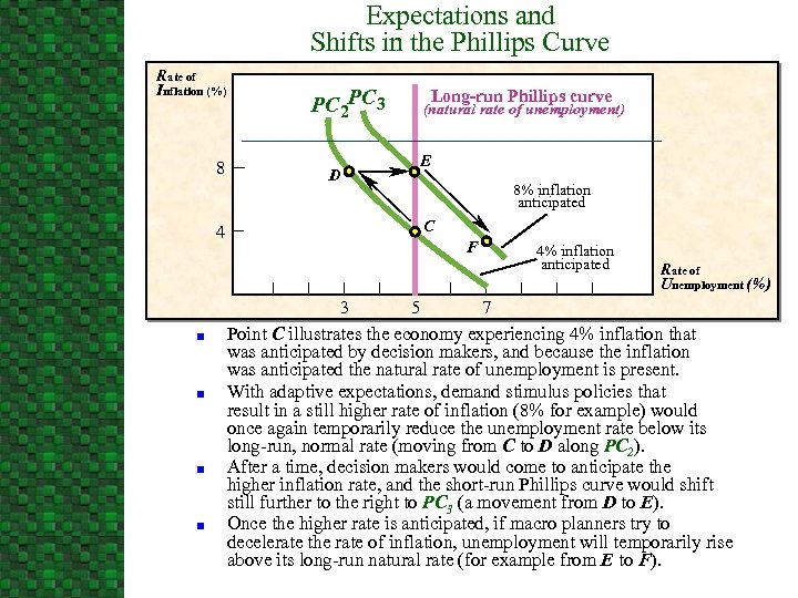Expectations and Shifts in the Phillips Curve Rate of Inflation (%) 8 4 n n PC 2 PC 3 D Long-run Phillips curve (natural rate of unemployment) E 8% inflation anticipated C F 4% inflation anticipated Rate of Unemployment (%) 3 5 7 Point C illustrates the economy experiencing 4% inflation that was anticipated by decision makers, and because the inflation was anticipated the natural rate of unemployment is present. With adaptive expectations, demand stimulus policies that result in a still higher rate of inflation (8% for example) would once again temporarily reduce the unemployment rate below its long-run, normal rate (moving from C to D along PC 2). After a time, decision makers would come to anticipate the higher inflation rate, and the short-run Phillips curve would shift still further to the right to PC 3 (a movement from D to E). Once the higher rate is anticipated, if macro planners try to decelerate the rate of inflation, unemployment will temporarily rise above its long-run natural rate (for example from E to F).

Expectations and the Modern View of the Phillips Curve n There is exists no permanent tradeoff between inflation and unemployment. u u u n Demand stimulus will lead to inflation without permanently reducing unemployment below the natural rate. Like LRAS, the Long-Run Phillips Curve is vertical at the natural rate of unemployment. When inflation is greater than anticipated, unemployment falls below the natural rate. When the inflation rate is steady — neither rising nor falling — the actual rate of unemployment will equal the economy’s natural rate of unemployment.

The Phillips Curve and Macro-policy n n The early view that there was a trade-off between inflation and unemployment helped promote the more expansionary macro policy of the 1970 s. Rejection of this view during the 1980 s created an environment more conducive to price stability. u n In turn, the increase in price level stability contributed to the lower unemployment rates of the 1990 s. In the long-run, expansionary policy in pursuit of lower unemployment leads to higher rates of both inflation and unemployment.

The Phillips Curve and Macro-policy n There are two important lessons to be learned from the Phillips curve era: u u n Expansionary macro policy will not reduce the rate of unemployment, at least not for long. Macro policy, particularly monetary policy, can achieve persistently low rates of inflation, which will help promote low rates of unemployment. There is no inconsistency between low (and stable) rates of inflation and low rates of unemployment.