87eee88c7db4d2abec3c45dc49401f83.ppt
- Количество слайдов: 20
A Disequilibrium Model of the Housing Market: Implicit Selling Time as a Signal of the Optimal Holding Period and Buyer Valuations Eric Levin and Gwilym Pryce Department of Urban Studies University of Glasgow European real estate society conference Stockholm 24 to 27 June 2009
Why are falling house prices associated with a large increase in the inventory of unsold homes and an accompanying decline in sales volume? Existing explanations for these phenomena include 1. psychological reluctance to realize loss when the market values of houses fall below the prices that the current owners paid for them 2. the negative equity effect on the owner of a property with a high loan-to-value ratio who requires the proceeds from the sale of the existing house to provide the down payment for the next home. Our analysis, while not precluding these factors, provides a simple statistical explanation that requires only the minimal assumption of a distribution of valuations for potential buyers and sellers that is not directly observable by house market participants.

The source of the problem - valuation varies between individuals For most markets unplanned inventory movement signals excess demand. manufacturers – look at the unsold inventory every week market-makers - unexpected inventory movement signals excess demand The uniqueness of each house with respect to location and characteristics prevents institutional arrangements establishing a market-clearing price. The distribution of intra-marginal valuations becomes central in explaining price, time on the market and large swings in unsold inventories of unsold houses over the cycle.
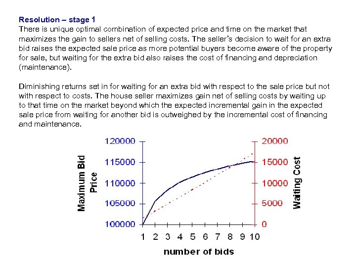
Resolution – stage 1 There is unique optimal combination of expected price and time on the market that maximizes the gain to sellers net of selling costs. The seller’s decision to wait for an extra bid raises the expected sale price as more potential buyers become aware of the property for sale, but waiting for the extra bid also raises the cost of financing and depreciation (maintenance). Diminishing returns set in for waiting for an extra bid with respect to the sale price but not with respect to costs. The house seller maximizes gain net of selling costs by waiting up to that time on the market beyond which the expected incremental gain in the expected sale price from waiting for another bid is outweighed by the incremental cost of financing and maintenance.
But this first stage of the analysis is limited by the assumptions that the waiting time per bid is exogenously given and that the population of potential buyers and sellers are informed about the mean and standard deviation of the valuation distribution.
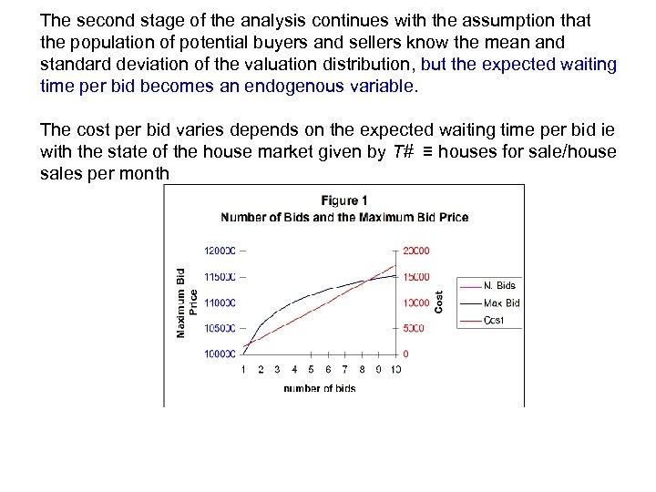
The second stage of the analysis continues with the assumption that the population of potential buyers and sellers know the mean and standard deviation of the valuation distribution, but the expected waiting time per bid becomes an endogenous variable. The cost per bid varies depends on the expected waiting time per bid ie with the state of the house market given by T# ≡ houses for sale/house sales per month
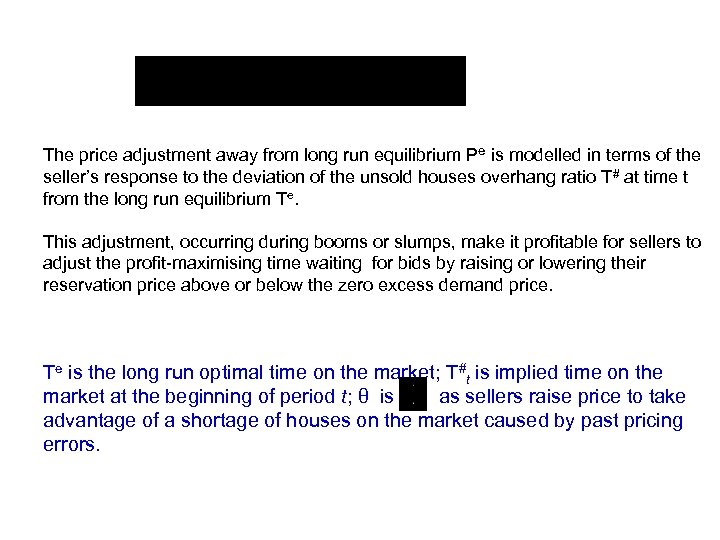
The price adjustment away from long run equilibrium Pe is modelled in terms of the seller’s response to the deviation of the unsold houses overhang ratio T# at time t from the long run equilibrium Te. This adjustment, occurring during booms or slumps, make it profitable for sellers to adjust the profit-maximising time waiting for bids by raising or lowering their reservation price above or below the zero excess demand price. Te is the long run optimal time on the market; T#t is implied time on the market at the beginning of period t; θ is as sellers raise price to take advantage of a shortage of houses on the market caused by past pricing errors.
The mean of the valuation distribution μ also changes over time. Changes in the zero excess demand price Pe over time consist of two components. The first component is publicly available new information that alters expectations about future house prices. The second component is the perception of new private information. Private information is defined as information that is known to informed market participants but is not generally available to sellers and estate agents. Estate agents cannot directly observe the private information component, but they are able to observe its effect on unanticipated movements in T#t.

where: is the change in the zero excess demand price between the beginning of period t-1 and the beginning of period t attributable to private information; and t is the shift in the zero excess demand market price attributable to public news incorporated into the price since the last period.

Substituting Equation (11) into Equation (10) gives: This eliminates the unobservable Pte from the expression
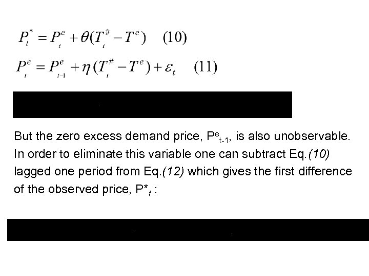
But the zero excess demand price, Pet-1, is also unobservable. In order to eliminate this variable one can subtract Eq. (10) lagged one period from Eq. (12) which gives the first difference of the observed price, P*t :

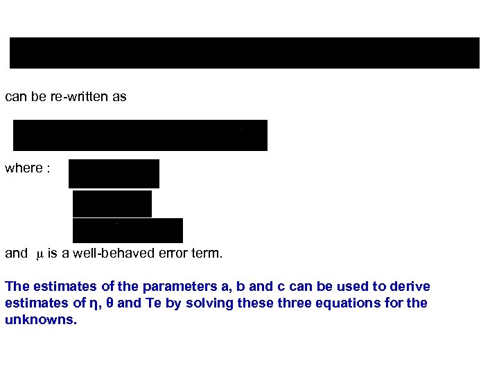
can be re-written as where : and is a well-behaved error term. The estimates of the parameters a, b and c can be used to derive estimates of η, θ and Te by solving these three equations for the unknowns.
Data The house price data, measured as the average price per room for properties sold on the second Thursday of each month, and selling time data was provided by he Glasgow Solicitors Property Centre (GSPC), a consortium of estate agents in the Strathclyde region of Scotland for the period 1999– 2007.

Monthly Change in House Prices The monthly change in price is calculated as (av. Pt - av. Pt-1)/av. Pt-1 where av. Pt is the average GSPC sale price per room over the last three months. Time on the Market T# GSPC also provided sales per month and the number of unsold houses for sale on the second Thursday of each month between 1999 and 2007. T# for each month was calculated as the average number of unsold houses for sale divided by the number of sales over the last three months.

Results The regression estimation equation differs from Eq (14). First, the dependent variable is expressed as a proportional change rather than an absolute change in order to eliminate bias caused by effects of inflation over the sample period. Second, a logarithmic relationship was used to take account of the curvature of d. P/d. T# as a function of T# associated with the curvature of the number of bids as a function of time as shown in Figures 1 and 2. Third, a moving average term was added to allow for an error correction term. The parameters of interest in (14) were estimated by fitting the following model for the monthly data set 1999: 2 to 2007: 11

where is the growth in the price of houses in Glasgow in month t, a is a constant, MA(1) is a moving average and it is a random error term. The estimates of (16) are shown in Table 2.


Now substitute the estimated parameter values into (15) to give: Start with the effect of historical pricing errors. θ measures the price response to the overhang of unsold houses during booms or slumps that make it profitable for sellers to adjust the profit maximising waiting time for bids by raising or lowering their reservation price above or below the zero excess demand price. The profit maximising price P* is 2. 5% higher when unsold houses for sales to sales ratio falls by unity. Turning to the excess demand price adjustment, η defines the slope of the long run excess demand curve d. Pe/d. T#. A half percent price rise is required to eliminate excess demand when the implied time on the market (ratio of unsold houses for sale to sales) shortens by unity, for example from the sample mean of 2. 3 months to 1. 3. Turning to the long run equilibrium level of Tt#, the constant term in Table 2 can be substituted into (15) to give That is, the estimated unobservable long run equilibrium implied time on the market Te is 3. 7 months.
87eee88c7db4d2abec3c45dc49401f83.ppt