A Combination Method for Generating Interpolants Greta Yorsh

A Combination Method for Generating Interpolants Greta Yorsh Madan Musuvathi Tel Aviv University, Israel Microsoft Research, Redmond, US CAV’ 05 1

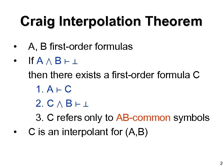
Craig Interpolation Theorem • • • A, B first-order formulas If A B then there exists a first-order formula C 1. A C 2. C B 3. C refers only to AB-common symbols C is an interpolant for (A, B) 2

Motivation • Abstraction – forget some information about the system – preserve enough information to show that an error state is not reachable • Interpolation – forget some information about A – preserve enough information to show that B is unsatisfiable 3

Motivation • Bounded Model Checking [Mc. Millan, CAV’ 03] – abstraction of reachable states – completeness C initial reachable in k steps A-part error B-part 4

Motivation • Bounded model checking [Mc. Millan, CAV’ 03] – propositional (hardware) and first-order (software) • Predicate abstraction refinement [HJMS, POPL’ 04] – first-order • Computation of the abstract transition relation [Mc. Millan et al. , CAV’ 05] – propositional • Exploit prover’s ability to focus on relevant facts 5

Interpolant Generation • Craig interpolation theorem [’ 57] – (full) first-order logic – existence of interpolants (cut elimination) • Pudlak [‘ 95], Krajicek [’ 95] – propositional logic • Pudlak [‘ 95] – linear inequalities (LI) • Mc. Millan [TACAS’ 04] – uninterpreted functions (UF) – the combinated theory of UF and LI (with boolean combinations) 6

Nelson-Oppen Combination Method • Satisfiability in a combined theory [’ 79] • Given – P 1 is a decision procedure for satisfiability in T 1 – P 2 is a decision procedure for satisfiability in T 2 • Combines P 1 and P 2 into a decision procedure for satisfiability in the combined theory T = T 1 T 2 7

Interpolant Generation in Combined Theory • Given – P 1 interpolant generation procedure for T 1 – P 2 interpolant generation procedure for T 2 • How to combine P 1 and P 2 into an interpolant generation procedure for the combined theory T = T 1 T 2 ? 8

Outline • • • Notations Partial interpolants Example Equality-interpolating theories Conclusions 9

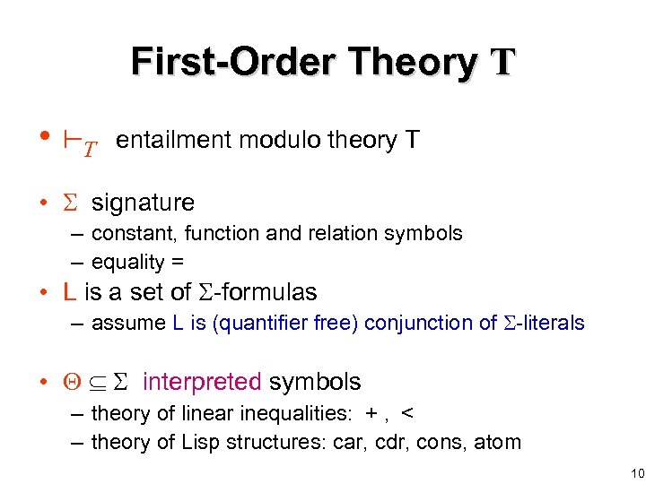
First-Order Theory T • T entailment modulo theory T • signature – constant, function and relation symbols – equality = • L is a set of -formulas – assume L is (quantifier free) conjunction of -literals • interpreted symbols – theory of linear inequalities: + , < – theory of Lisp structures: car, cdr, cons, atom 10

Example Theories • UF – Uninterpreted Functions – contains uninterpreted function symbols: f, g, . . . – is empty – example: f(a, b) = g(c) • LI - Linear Inequalities – contains + , < , 0, 1, 2, . . . – example: a < b + 2*c • Lisp structures – = { car, cdr, cons, atom } – example: car(a) = cons(car(b), cdr(c)) 11

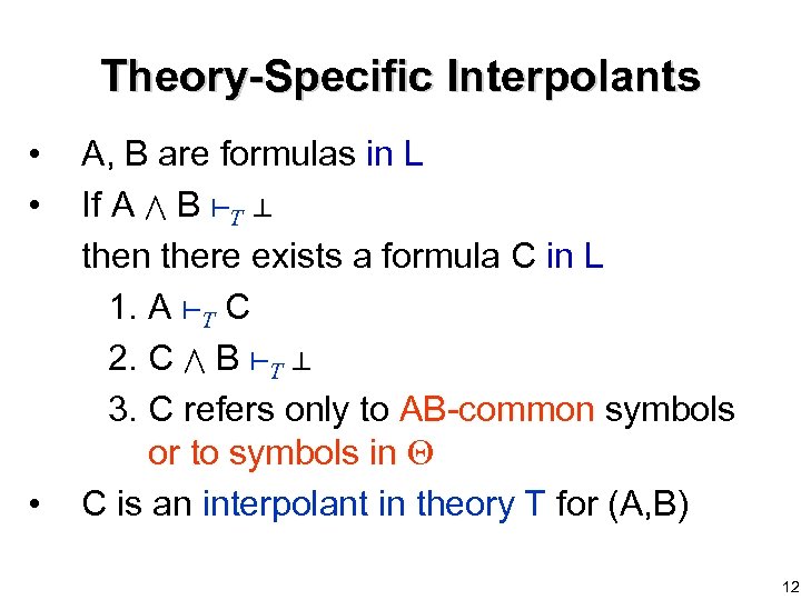
Theory-Specific Interpolants • • • A, B are formulas in L If A B T then there exists a formula C in L 1. A T C 2. C B T 3. C refers only to AB-common symbols or to symbols in C is an interpolant in theory T for (A, B) 12

Example: Lisp Structures A car(a) = c 2 c 3 = cdr(a) a = c 1 atom(c 1) B (b = cons(c 2, c 3)) c 1 = b – A-local symbols: a, car, cdr, atom – B-local symbols: b, cons – AB-common symbols: c 1, c 2, c 3 – is { car, cdr, cons, atom } • Interpolant for (A, B) in Lisp theory is c 1 = cons(c 2, c 3) 13

Combined Theory T • First-order theory T defined as a combination of T 1 and T 2 – T is T 1 T 2 (union of axioms / intersection of sets of models) – is 1 1 – is 1 2 – disjoint signatures: 1 2 is { = } 14

Interpolants in Combined Theory • A is (f(x 1) + x 2 = x 3) (f(y 1) + y 2 = y 3) (y 1 x 1) • B is (x 2 = g(b)) (y 2 = g(b)) (x 1 y 1) (x 3 < y 3) • Purify A and B separately – AUF ALI is the result of purify(A) – BUF BLI is the result of purify(B) T is UF LI A a 1 = f(x 1) UF a = f(y ) 2 1 B x 2 = g(b) y 2 = g(b) a 1 + x 2 = x 3 LI a 2 + y 2 = y 3 y 1 x 1 y 1 x 3 < y 3 15

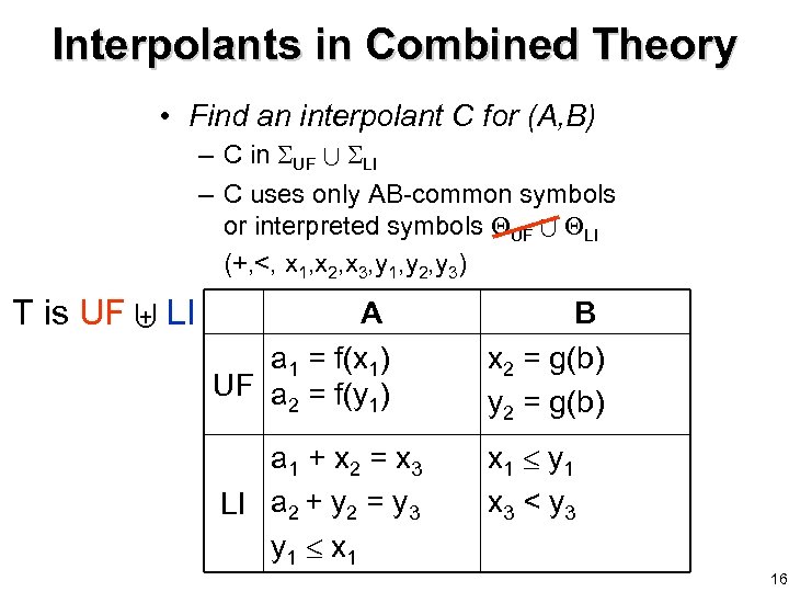
Interpolants in Combined Theory • Find an interpolant C for (A, B) – C in UF LI – C uses only AB-common symbols or interpreted symbols UF LI (+, <, x 1, x 2, x 3, y 1, y 2, y 3) T is UF LI A a 1 = f(x 1) UF a = f(y ) 2 1 B x 2 = g(b) y 2 = g(b) a 1 + x 2 = x 3 LI a 2 + y 2 = y 3 y 1 x 1 y 1 x 3 < y 3 16

Interpolant Generation in Combined Theory • Given – P 1 is a decision procedure for T 1 – P 2 is a decision procedure for T 2 • Combine P 1 and P 2 into an interpolant generation procedure for the combined theory T = T 1 T 2 17

Requirements • Requirement on procedure P 1 (same for P 2) – P 1 is a decision procedure for satisfiability of T 1 – if input is satisfiable P 1 generates a new consequence (equality between variables) – if input of the form A B is unsatisfiable in T 1, P 1 generates an interpolant for A and B in T 1 • Requirement on T 1 (and T 2) – stably-infinite – convex – equality-interpolating 18

Equality Propagation AUF a 1 = f(x 1) a 2 = f(y 1) BUF x 2 = g(b) y 2 = g(b) ALI a 1 + x 2 = x 3 a 2 + y 2 = y 3 y 1 x 1 BLI x 1 y 1 x 3 < y 3 a 1=a 2 [ ? ] PUF x 2=y 2 [ ? ] x 1=y 1 [ ? ] PLI [ CLI ] CLI is interpolant for ALI (a 1=a 2) and BLI (x 2=y 2) CLI is x 2 -y 2 = x 3 -y 3 CLI is not an interpolant for (A, B) 19

Observation • CLI is interpolant for ALI (a 1=a 2) and BLI (x 2=y 2) • CLI is not an interpolant for (A, B) – ALI (a 1=a 2) T CLI but A T CLI – a 1=a 2 follows from A B, but not A alone • How to “lift” CLI to an interpolant for (A, B) ? 20

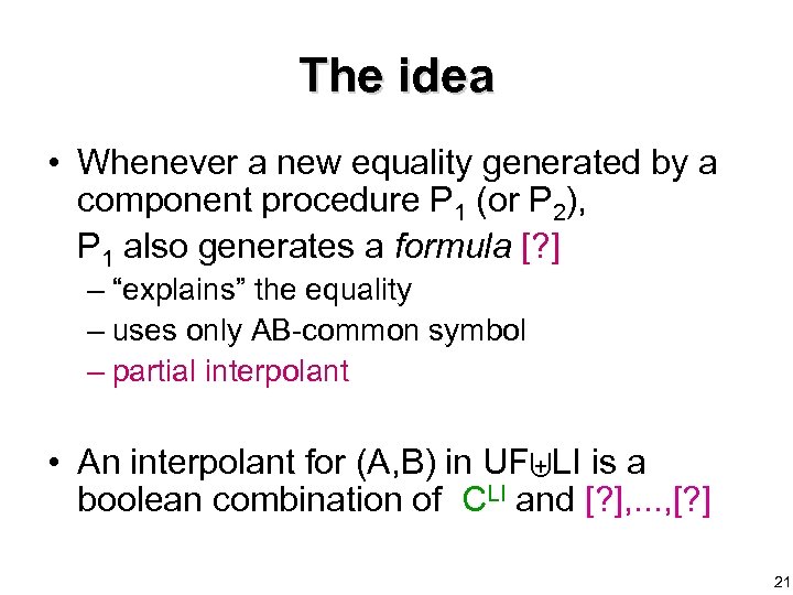
The idea • Whenever a new equality generated by a component procedure P 1 (or P 2), P 1 also generates a formula [? ] – “explains” the equality – uses only AB-common symbol – partial interpolant • An interpolant for (A, B) in UF LI is a boolean combination of CLI and [? ], . . . , [? ] 21

Theory-Specific Partial Interpolants • A 1 B 1 T 1 x=y • A 1 B 1 (x=y) T 1 A 1 B 1 P 1 x=y 22

Theory-Specific Partial Interpolants • A 1 B 1 T 1 x=y • A 1 B 1 (x=y) T 1 • CT 1(x=y) a theory-specific partial interpolant of x=y for A 1 and B 1 in theory T 1 – interpolant for A 1 and B 1 (x=y) if x, y B-local AB-common – interpolant for A 1 (x=y) and B 1 if x, y A-local AB-common A 1 B 1 x=y P 1 [ CT 1 ] 23

Partial Interpolants (a=a’) A 1 B 1 (b=b’) [ C(a=a’) ] • CT 1(x=y) is a theory-specific partial interpolant of x=y for A 1 (a=a’) and B 1 (b=b’) in theory T 1 [ C(b=b’) ] P 1 • C(x=y) a partial interpolant x=y [ CT 1(x=y) ] of x=y for A and B in T 1 T 2 is a boolean combination of [? ] CT 1(x=y) and C(a=a’) and C(b=b’) 24

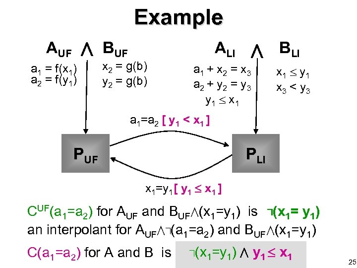
Example AUF a 1 = f(x 1) a 2 = f(y 1) BUF ALI x 2 = g(b) y 2 = g(b) a 1 + x 2 = x 3 a 2 + y 2 = y 3 y 1 x 1 BLI x 1 y 1 x 3 < y 3 a 1=a 2 [ y 1 < x 1 ] PUF PLI x 1=y 1 [ y 1 x 1 ] CUF(a 1=a 2) for AUF and BUF (x 1=y 1) is (x 1= y 1) an interpolant for AUF (a 1=a 2) and BUF (x 1=y 1) C(x =y C(a 1=a 2) for A and B is CUF(a 1=a 2) y 1 1 x 1 1) 25

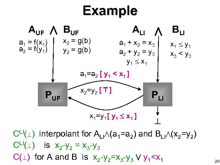
Example AUF a 1 = f(x 1) a 2 = f(y 1) BUF ALI x 2 = g(b) y 2 = g(b) a 1 + x 2 = x 3 a 2 + y 2 = y 3 y 1 x 1 BLI x 1 y 1 x 3 < y 3 a 1=a 2 [ y 1 < x 1 ] PUF x 2=y 2 [ ] x 1=y 1 [ y 1 x 1 ] PLI CLI( ) interpolant for ALI (a 1=a 2) and BLI (x 2=y 2) CLI( ) is x 2 -y 2 = x 3 -y 3 C( ) for A and B is x 2 -y 2=x 3 -y 3 y 1<x 1 26

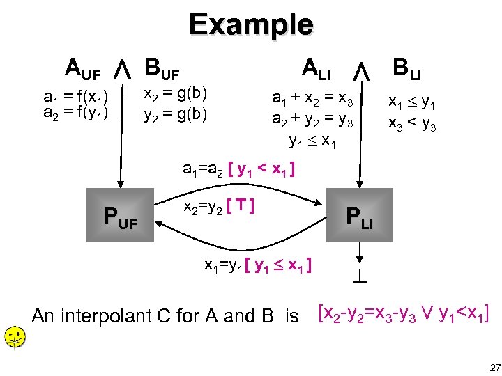
Example AUF a 1 = f(x 1) a 2 = f(y 1) BUF ALI x 2 = g(b) y 2 = g(b) a 1 + x 2 = x 3 a 2 + y 2 = y 3 y 1 x 1 BLI x 1 y 1 x 3 < y 3 a 1=a 2 [ y 1 < x 1 ] PUF x 2=y 2 [ ] x 1=y 1 [ y 1 x 1 ] PLI An interpolant C for A and B is [x 2 -y 2=x 3 -y 3 y 1<x 1] 27

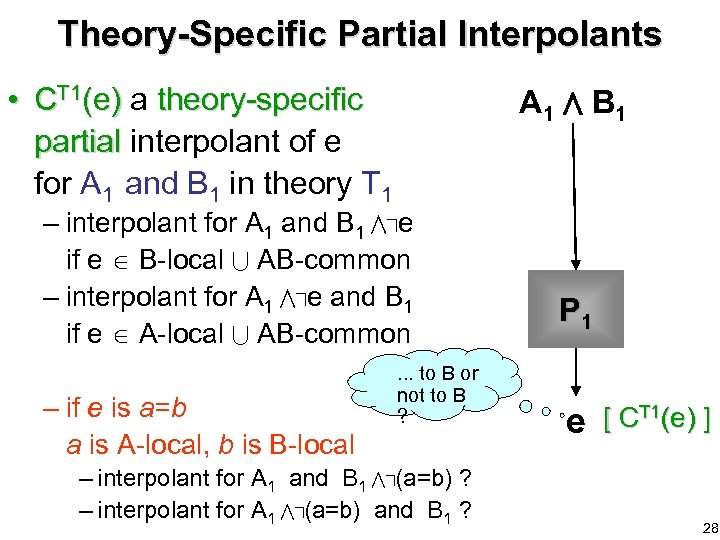
Theory-Specific Partial Interpolants • CT 1(e) a theory-specific partial interpolant of e for A 1 and B 1 in theory T 1 A 1 B 1 – interpolant for A 1 and B 1 e if e B-local AB-common – interpolant for A 1 e and B 1 if e A-local AB-common – if e is a=b a is A-local, b is B-local . . . to B or not to B ? – interpolant for A 1 and B 1 (a=b) ? – interpolant for A 1 (a=b) and B 1 ? P 1 e [ CT 1(e) ] 28

Equality-Interpolating Theory • If A B T (a = b) – a is A-local, b is B-local • then there exists a term t – A B T (a = t) (t = b) – t refers to AB-common symbols only • Equality-interpolating: UF, LI, Lisp – easy to extend the existing decision procedures to generate such terms t 29

Requirements • Requirement on P 1 (and P 2) – P 1 is a decision procedure for satisfiability of T 1 – if input is satisfiable P 1 generates a new consequence (equality between variables) – if input of the form A B is unsatisfiable in T 1, P 1 generates an interpolant for A and B in T 1 • Requirement on T 1 (and T 2) – stably-infinite – convex – equality-interpolating 30

Summary • A method for generating interpolants for combined theories – – interpolant-generation procedures P 1, P 2 used as black-boxes on top of a Nelson-Oppen procedure propagate partial interpolants equality-interpolating theories • Can be integrated within existing tools – Simplify, Verifun, ICS, CVCLite, Zap • Extensions – arbitrary quantifier-free formulas, non-convex theories, non-disjoint signatures, quantifiers • Application to software model-checking • More support for operations modulo theories – join, widening, predicate abstraction, counter-example generation 31