5a294dea3a6e27d42dbff48a323d5949.ppt
- Количество слайдов: 96


A Brief Survey of Machine Learning

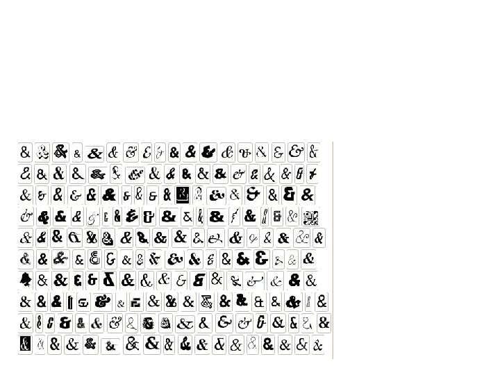
Example: Various Fonts classification

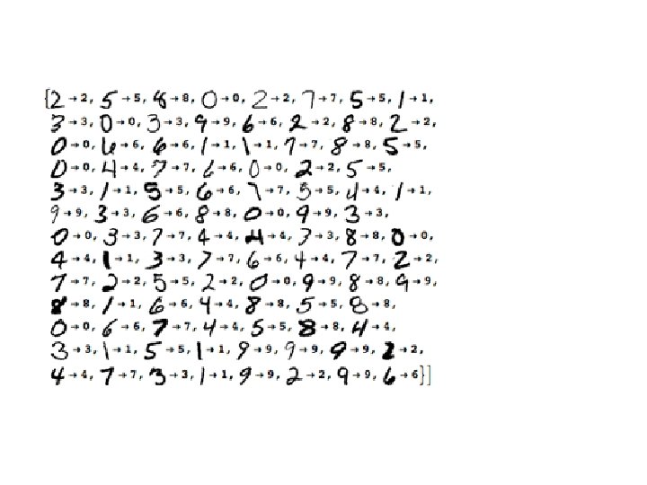
Example: Handwritten Digits Recognition

Example Abstract Images

Training Examples: Class 1 Training Examples: Class 2 Test example: Class = ?

Machine Learning Lectures Outline: what we will discuss?

ML Lectures Outline: what we will discuss? • We know already several methods of machine learning. • What are general principles? • Can we create improved methods? • What are examples of applications of Machine Learning?

ML Lectures Outline: what we will discuss? • Why machine learning? • Brief Tour of Machine Learning – A case study – A taxonomy of learning – Intelligent systems engineering: specification of learning problems • Issues in Machine Learning – Design choices – The performance element: intelligent systems • Some Applications of Learning – Database mining, reasoning (inference/decision support), acting – Industrial usage of intelligent systems – Robotics

What is Learning?

What is Learning? definitions • “Learning denotes changes in a system that. . . enable a system to do the same task more efficiently the next time. ” -- Herbert Simon • “Learning is constructing or modifying representations of what is being experienced. ” - Ryszard Michalski • “Learning is making useful changes in our minds. ” -- Marvin Minsky

Why Machine Learning? What ML can do? • Discovers new things or structures that are unknown to humans – Examples: – Data mining, – Knowledge Discovery in Databases • Fills in skeletal or incomplete specifications about a domain – Large, complex AI systems cannot be completely derived by hand – They require dynamic updating to incorporate new information. – Learning new characteristics: – 1. expands the domain or expertise – 2. lessens the "brittleness" of the system • Using learning, the software agents can adapt to: – to their users, – to other software agents, – to the changing environment.
 records")
Why Machine Learning? • New Computational Capability – Database mining: – converting (technical) records into knowledge – Self-customizing programs: – learning news filters, – adaptive monitors – Learning to act: – robot planning, – control optimization, – decision support – Applications that are hard to program: – automated driving, – speech recognition

Why Machine Learning? • Better Understanding of Human Learning and Teaching – Understand improve efficiency of human learning – Use to improve methods for teaching and tutoring people – e. g. , better computer-aided instruction. (can our robot-head teach English? ) – Cognitive science: theories of knowledge acquisition (e. g. , through practice) – Performance elements: reasoning (inference) and recommender systems • Time is Right – Recent progress in algorithms and theory – Rapidly growing volume of online data from various sources – Available computational power – Growth and interest of learning-based industries (e. g. , data mining/KDD)

A General Model of Learning Agents

Disciplines relevant to Machine Learning • Artificial Intelligence • Bayesian Methods • Cognitive Science • Computational Complexity Theory • Control Theory • Information Theory • Neuroscience • Philosophy • Psychology • Statistics PAC Formalism Mistake Bounds Optimization Learning Predictors Meta-Learning Entropy Measures MDL Approaches Optimal Codes Language Learning to Reason Bayes’s Theorem Missing Data Estimators Machine Learning Symbolic Representation Planning/Problem Solving Knowledge-Guided Learning Bias/Variance Formalism Confidence Intervals Hypothesis Testing Power Law of Practice Heuristic Learning Occam’s Razor Inductive Generalization ANN Models Modular Learning

Forms of Machine Learning • Supervised – Learns from examples which provide desired outputs for given inputs • Unsupervised – Learns patterns in input data when no specific output values are given • Reinforcement – Learns by an indication of correctness at end of some reasoning So far, we covered only Supervised Learning, but this knowledge will be also useful in Unsupervised and Reinforcement Learning
 to be considered")
Supervised Learning • Must have training data including – Inputs (features) to be considered in decision – Outputs (correct decisions) for those inputs • Inductive reasoning – Given a collection of examples of function f, return a function h that approximates f – Difficulty: many functions h may be possible Difficulty – Hope to pick function h that generalizes well – Tradeoff between the complexity of the hypothesis and the degree of fit to the data – Consider data modeling

Decision Trees, Decision Diagrams, Decompositions
 • Map features of situation to decision –")
Decision Trees or Decision Diagrams (DAG) • Map features of situation to decision – Example from a classification of unsafe acts: In general, branches of a tree can be combined to create a DAG (Directed Acyclic Graph)

Decision Trees, not only binary attributes and decisions • The actions can be more than only yes/no decisions of a classifier. • Relation to rule-based reasoning – Features of element used to classify element – Features of situation used to select action • Used as the basis for many “how to” books – How to identify type of snake? – Observable features of snake – How to fix an automobile? – Features related to problem and state of automobile – If features are understandable, the decision tree can be used to explain decision

Learning Decision Trees: classification versus regression • Types of Decision Trees – Learning a discrete-valued function is classification learning – Learning a continuous-valued function is regression • Assumption: use of Ockham’s razor will result in more general function – Want the smallest decision tree, but that is not tractable – Will be satisfied with smallish tree

Algorithm for Decision Tree Learning • Basic idea – Recursively select feature that splits data (most) unevenly – No need to use all features 1. Can be generalized to decomposition methods 2. Can be generalized to other types of trees, DAGs. • Heuristic approach (applied not only to trees) – Compare features for their ability to meaningfully split data – – Feature-value = greatest difference in average output value(s) * size of smaller subset Avoids splitting out individuals too early

MAIN FORMAT OF DATA for classification

Classification Terms • Data: A set of N vectors x – Features are parameters of x; x lives in feature space – May be 1. 2. 3. 4. 5. whole, raw images; parts of images; filtered images; statistics of images; or something else entirely • Labels: C categories; each x belongs to some ci • Classifier: Create formula(s) or rule(s) that will assign unlabeled data to correct category – Equivalent definition is to parametrize a decision surface in feature space separating category members plus the awareness that there’s a lot of data out there that the classifier may yet encounter

Example: Road classification

Features and Labels for Road Classification We want to classify for each pixel, does it belong to a road or not. • Feature vectors: 410 features/point over 32 x 20 grid – Color histogram [Swain & Ballard, 1991] (24 features) – 8 bins per RGB channel over surrounding 31 x 31 camera subimage – Gabor wavelets [Lee, 1996] (384) – Characterize texture with 8 -bin histogram of filter responses for – – – 2 phases, 3 scales, 8 angles over 15 x 15 camera subimage – Ground height, smoothness (2) – Mean, variance of laser height values • projecting to 31 x 31 camera subimage Labels derived from inside/outside relationship of feature point to road-delimiting polygon

Features and Labels for Road Classification 0° even 45° even 0° odd from Rasmussen, 2001 So for classification, the term “features” is commonly used, but you can think of these as the road analogs of attributes. Features are computed on a grid every 10 pixels horizontally and vertically the three Gabor filter scales correspond to kernel sizes of 6 x 6, 12 x 12, and 25 x 25

Key Classification Problems 1. What features to use? How do we extract them from the image? 2. Do we even have labels (i. e. , examples from each category)? 3. What do we know about the structure of the categories in feature space?

Theoretical Aspects of Learning Systems

Three Aspects of Learning Systems – 1. Models: – decision trees, – linear threshold units (winnow, weighted majority), – neural networks, – Bayesian networks (polytrees, belief networks, influence diagrams, HMMs), – genetic algorithms, – instance-based (nearest-neighbor) – 2. Algorithms (e. g. , for decision trees): – ID 3, – C 4. 5, – CART, – OC 1 – 3. Methodologies: – supervised, – unsupervised, – reinforcement; – knowledge-guided

What are the aspects of research on Learning? • 1. Theory of Learning – Computational learning theory (COLT): complexity, limitations of learning – Probably Approximately Correct (PAC) learning – Probabilistic, statistical, information theoretic results • 2. Multistrategy Learning: – Combining Techniques, – Knowledge Sources • 3. Create and collect Data: – Time Series, – Very Large Databases (VLDB), – Text Corpora • 4. Select good applications – Performance element: – classification, – decision support, – planning, – control – Database mining and knowledge discovery in databases (KDD) – Computer inference: learning to reason

Some Issues in Machine Learning • What Algorithms Can Approximate Functions Well? • How Do Learning System Design Factors Influence Accuracy? When? – Number of training examples – Complexity of hypothesis representation • How Do Learning Problem Characteristics Influence Accuracy? – Noisy data – Multiple data sources • What Are Theoretical Limits of Learnability? • How Can Prior Knowledge of Learner Help? • What Clues Can We Get From Biological Learning Systems? • How Can Systems Alter Their Own Representation?

Major Paradigms of Machine Learning

Major Paradigms of Machine Learning • Rote Learning – One-to-one mapping from inputs to stored representation. – "Learning by memorization. ” – Association-based storage and retrieval. • Clustering • Analogue – Determine correspondence between two different representations • Induction – Use specific examples to reach general conclusions • Discovery – Unsupervised, specific goal not given • Genetic Algorithms

Major Paradigms of Machine Learning • Neural Networks • Reinforcement – Feedback given at end of a sequence of steps. – Feedback can be positive or negative reward – Assign reward to steps by solving the credit assignment problem — – which steps should receive credit or blame for a final result?

The Inductive Learning Problem

The Inductive Learning Problem • Induce rules that extrapolate from a given set of examples – These rules should make “accurate” predictions about future examples. • Supervised versus Unsupervised learning – Learn an unknown function f(X) = Y, where: – X is an input example and – Y is the desired output. – Supervised learning implies we are given a training set of (X, Y) pairs by a "teacher. “ – Unsupervised learning means we are only given the Xs and some (ultimate) feedback function on our performance.

The Inductive Learning Problem • Concept learning – Called also Classification – Given a set of examples of some concept/class/category, determine if a given example is an instance of the concept or not. – If it is an instance, we call it a positive example. – If it is not, it is called a negative example.

Inductive Learning Framework • Raw input data from sensors are preprocessed to obtain a feature vector, X, that adequately describes all of the relevant features for classifying examples. • Each x is a list of (attribute, value) pairs. For example, X = [Person: Sue, Eye. Color: Brown, Age: Young, Sex: Female] • The number and names of attributes (aka features) is fixed (positive, finite). • Each attribute has a fixed, finite number of possible values. • Each example can be interpreted as a point in an n-dimensional feature space, where n is the number of attributes.

Example Learning to play Checkers

Specifying A Learning Problem • Learning = Improving with Experience at Some Task – Improve over task T, – with respect to performance measure P, – based on experience E. • Example: Learning to Play Checkers – T: play games of checkers – P: percent of games won in world tournament – E: opportunity to play against self • Refining the Problem Specification: Issues – What experience? – What exactly should be learned? – How shall it be represented? – What specific algorithm to learn it? • Defining the Problem Milieu – Performance element: – How shall the results of learning be applied? – How shall the performance element be evaluated? The learning system?

Example: Learning to Play Checkers • Type of Training Experience – Direct or indirect? – Teacher or not? – Knowledge about the game (e. g. , openings/endgames)? • Problem: Is Training Experience Representative (of Performance Goal)? • Software Design – Assumptions of the learning system: legal move generator exists – Software requirements: – generator, – evaluator(s), – parametric target function • Choosing a Target Function – Choose. Move: Board Move (action selection function, or policy) – V: Board R (board evaluation function) – Ideal target V; approximated target – Goal of learning process: operational description (approximation) of V

A Target Function for Learning to Play Checkers • Possible Definition – If b is a final board state that is won, then V(b) = 100 – If b is a final board state that is lost, then V(b) = -100 – If b is a final board state that is drawn, then V(b) = 0 – If b is not a final board state in the game, then V(b) = V(b’) where b’ is the best final board state that can be achieved starting from b and playing optimally until the end of the game – Correct values, but not operational • Choosing a Representation for the Target Function – Collection of rules? – Neural network? – Polynomial function (e. g. , linear, quadratic combination) of board features? – Other? • A Representation for Learned Function – – bp/rp = number of black/red pieces; bk/rk = number of black/red kings; = number of black/red pieces threatened (can be taken on next turn) bt/rt

A Training Procedure for Learning to Play Checkers • Obtaining Training Examples – – the learned function – • the target function the training value One Rule For Estimating Training Values: – • Choose Weight Tuning Rule – Least Mean Square (LMS) weight update rule: REPEAT • Select a training example b at random • Compute the error(b) for this training example • For each board feature fi, update weight wi as follows: where c is a small, constant factor to adjust the learning rate

Design Choices for Learning to Play Checkers Determine Type of Training Experience Games against experts Games against self Table of correct moves Determine Target Function Board move Board value Determine Representation of Learned Function Polynomial Linear function of six features Artificial neural network Determine Learning Algorithm Gradient descent Completed Design Linear programming

Supervised Learning

Evaluating Supervised Learning Algorithms
 2.")
Evaluating Supervised Learning Algorithms 1. Collect a large set of examples (input/output pairs) 2. Divide into two disjoint sets 1. Training data 2. Testing data 3. Apply learning algorithm to training data, generating a hypothesis h 4. Measure % of examples in the testing data that are successfully classified by h (or amount of error for continuously valued outputs) 5. Repeat above steps for different sizes of training sets and different randomly selected training sets

Supervised Concept Learning • Given a training set of positive and negative examples of a concept – Usually each example has a set of features/attributes • Construct a description that will accurately classify whether future examples are positive or negative. • That is, – learn some good estimate of function f – given a training set {(x 1, y 1), (x 2, y 2), . . . , (xn, yn)} – where each yi is either + (positive) or - (negative). – f is a function of the features/attributes

Supervised Learning: Assessing Classifier Performance • Bias: Accuracy or quality of classification • Variance: Precision or specificity—how stable is decision boundary for different data sets? – Related to generality of classification result Overfitting to data at hand will often result in a very different boundary for new data

Supervised Learning: Procedures • Validation: Split data into training and test set – Training set: Labeled data points used to guide parametrization of classifier – % misclassified guides learning – Test set: Labeled data points left out of training procedure – % misclassified taken to be overall classifier error • m-fold Cross-validation – Randomly split data into m equal-sized subsets – Train m times on m - 1 subsets, test on left-out subset – Error is mean test error over left-out subsets • Jackknife: Cross-validation with 1 data point left out – Very accurate; variance allows confidence measuring

k-Nearest Neighbor Classification – For a new point, grow sphere in feature space until k labeled points are enclosed – Labels of points in sphere vote to classify – Low bias, high variance: No structure assumed from Duda et al.

Inductive Learning by Nearest-Neighbor Classification • One simple approach to inductive learning is to save each training example as a point in feature space • Classify a new example by giving it the same classification (+ or -) as its nearest neighbor in Feature Space. – 1. A variation involves computing a weighted sum of class of a set of neighbors – where the weights correspond to distances – 2. Another variation uses the center of class • The problem with this approach is that it doesn't necessarily generalize well if the examples are not well "clustered. "
 = w. T x + w 0 – w")
Linear Discriminants • Basic: g(x) = w. T x + w 0 – w is weight vector, x is data, w 0 is bias or threshold weight – Number of categories – Two: Decide c 1 if g(x) < 0, c 2 if g(x) > 0. g(x) = 0 is decision surface—a hyperplane when g(x) linear – Multiple: Define C functions gi(x) = w. T xi + wi 0. Decide ci if gi(x) > gj(x) for all j i • Generalized: g(x) = a. T y – Augmented form: y = (1, x. T)T, a = (w 0, w. T)T – Functions yi = yi(x) can be nonlinear—e. g. , y = (1, x, x 2)T

Separating Hyperplane in Feature Space from Duda et al.

Computing Linear Discriminants • Linear separability: Some a exists that classifies all samples correctly • Normalization: If yi is classified correctly when a. T yi < 0 and its label is c 1, simpler to replace all c 1 -labeled samples with their negation – This leads to looking for an a such that a. T yi > 0 for all of the data • Define a criterion function J(a) that is minimized if a is a solution. – Then gradient descent on J (for example) leads to a discriminant

Criterion Functions • Idea: – J = Number of misclassified data points. – But only piecewise continuous Not good for gradient descent • Approaches to create criterion functions – Perceptron: Jp(a) = y Y (-a. T y), where Y(a) is the set of samples misclassified by a – Proportional to sum of distances between misclassified samples and decision surface – Relaxation: Jr(a) = ½ y Y (a. T y - b)2 / ||y||2, where Y(a) is now set of samples such that a. T y b – Continuous gradient; J not so flat near solution boundary – Normalize by sample length to equalize influences

Non-Separable Data: Error Minimization • Perceptron, Relaxation assume separability—won’t stop otherwise – Only focus on erroneous classifications • Idea: Minimize error over all data • Try to solve linear equations rather than linear inequalities: a. T y = b Minimize i (a. T yi – bi)2 • Solve batch with pseudoinverse or iteratively with Widrow-Hoff/LMS gradient descent • Ho-Kashyap procedure picks a and b together

Other Linear Discriminants • Winnow: Improved version of Perceptron – Error decreases monotonically – Faster convergence • Appropriate choice of b leads to Fisher’s Linear Discriminant (used in “Vision-based Perception for an Autonomous Harvester, ” by Ollis & Stentz) • Support Vector Machines (SVM) – Map input nonlinearly to higher-dimensional space (where in general there is a separating hyperplane) – Find separating hyperplane that maximizes distance to nearest data point

Neural Networks

Neural Networks • Many problems require a nonlinear decision surface • Idea: Learn linear discriminant and nonlinear mapping functions yi(x) simultaneously • Feedforward neural networks are multi-layer Perceptrons – Inputs to each unit are summed, bias added, put through nonlinear transfer function • Training: Backpropagation, a generalization of LMS rule

Neural Network Structure
![Neural Networks in Matlab net = newff(minmax(D), [h o], {'tansig', 'tansig'}, 'traincgf'); net =](https://present5.com/presentation/5a294dea3a6e27d42dbff48a323d5949/image-65.jpg "Neural Networks in Matlab net = newff(minmax(D), [h o], {'tansig', 'tansig'}, 'traincgf'); net =")
Neural Networks in Matlab net = newff(minmax(D), [h o], {'tansig', 'tansig'}, 'traincgf'); net = train(net, D, L); test_out = sim(net, test. D); where: D is training data feature vectors (row vector) L is labels for training data test. D is testing data feature vectors h is number of hidden units o is number of outputs
: Pomerleau et")
Neural Network Learning • Autonomous Learning Vehicle In a Neural Net (ALVINN): Pomerleau et al – http: //www. cs. cmu. edu/afs/cs/project/alv/member/www/projects/ALVINN. html – Drives 70 mph on highways

Principal Component Analysis
 can reduce dimensionality of feature space More")
Dimensionality Reduction • Functions yi = yi(x) can reduce dimensionality of feature space More efficient classification • If chosen intelligently, we won’t lose much information and classification is easier • Common methods – Principal components analysis (PCA): Maximize total “scatter” of data – Fisher’s Linear Discriminant (FLD): Maximize ratio of between-class scatter to within-class scatter

Principal Component Analysis • Orthogonalize feature vectors so that they are uncorrelated • Inverse of this transformation takes zero mean, unit variance Gaussian to one describing covariance of data points • Distance in transformed space is Mahalanobis distance • By dropping eigenvectors of covariance matrix with low eigenvalues, we are essentially throwing away least important dimensions

PCA

Dimensionality Reduction: PCA vs. FLD from Belhumeur et al. , 1996
 • Given cropped images {I} of faces")
Face Recognition (Belhumeur et al. , 1996) • Given cropped images {I} of faces with different lighting, expressions • Nearest neighbor approach equivalent to correlation (I’s normalized to 0 mean, variance 1) – Lots of computation, storage • PCA projection (“Eigenfaces”) – Better, but sensitive to variation in lighting conditions • FLD projection (“Fisherfaces”) – Best (for this problem)
")
Bayesian Decision Theory: Classification with Known Parametric Forms • Sometimes we know (or assume) that the data in each category is drawn from a distribution of a certain form—e. g. , a Gaussian • Then classification can be framed as simply a nearest-neighbor calculation, but with a different distance metric to each category—i. e. , the Mahalanobis distance for Gaussians

Decision Surfaces for Various 2 -Gaussian Situations from Duda et al.

Example: Color-based Image Comparison • Per image: e. g. , histograms from Image Processing lecture • Per pixel: Sample homogeneously-colored regions… – Parametric: Fit model(s) to pixels, threshold on distance (e. g. , Mahalanobis) – Non-parametric: Normalize accumulated array, threshold on likelihood • For a given homogeneous region, the first component of the prediction it makes about the image concerns its color. • In early work, I developed a novel way of defining an object’s color by sampling pixels from it, fitting an ellipsoid to those pixels’ colorspace projection using principal components analysis, and quantifying color similarity by the Mahalanobis distance, as you see here, where brighter pixels are more orange.

Color Similarity: RGB Mahalanobis Distance PCA-fitted ellipsoid Sample
![Non-parametric Color Models courtesy of G. Loy Skin chrominance points Smoothed, [0, 1]-normalized](https://present5.com/presentation/5a294dea3a6e27d42dbff48a323d5949/image-77.jpg "Non-parametric Color Models courtesy of G. Loy Skin chrominance points Smoothed, [0, 1]-normalized")
Non-parametric Color Models courtesy of G. Loy Skin chrominance points Smoothed, [0, 1]-normalized

Non-parametric Skin Classification courtesy of G. Loy
 – “Weak learners”:")
Other Methods • Boosting – Ada. Boost (Freund & Schapire, 1997) – “Weak learners”: Classifiers that do better than chance – Train m weak learners on successive versions of data set with misclassifications from last stage emphasized – Combined classifier takes weighted average of m “votes” • Stochastic search (think particle filtering) – Simulated annealing – Genetic algorithms

Unsupervised Learning

Unsupervised Learning • Used to characterize/explain the key features of a set of data – No notion of desired output – Example: identifying fast-food vs. fine-dining restaurants when classes are not known ahead of time • Techniques – Clustering (k means, HAC) – Self-Organizing Maps – Gaussian Mixture Models • More on this topic in Project 3

Unsupervised Learning • May know number of categories C, but not labels • If we don’t know C, how to estimate? – Occam’s razor (formalized as Minimum Description Length, or MDL, principle): Favor simpler classifiers over more complex ones – Akaike Information Criterion (AIC) • Clustering methods – k-means – Hierarchical – Etc.

k-means Clustering • Initialization: Given k categories, N points. • Pick k points randomly; these are initial means 1, …, k 1. Classify N points according to nearest i 2. Recompute mean i of each cluster from member points 3. If any means have changed, goto (1)

Example: 3 -means Clustering image segmentation—say, on the basis of color —is an obvious application here from Duda et al. Convergence in 3 steps

Reinforcement Learning

Reinforcement Learning • Many large problems do not have desired outputs that can be used as training data • Process – Agent (system) performs a set of actions – Agent occasionally receives a reward to indicate something went right or penalty to indicate something went wrong – Agent has to learn relationship between the model of the situation, the chosen actions, and the rewards/penalties

Analogy to Animal Training • We cannot tell our pets what is right and wrong in (preconditions, action) pairs • Instead we reward good behavior (giving treats) and penalize bad behavior (spraying water or loud noise) • Pet has to learn when and where what is appropriate – Can result in incorrect interpretations (go in corner vs. go outside) • Difficulty: what of the prior/recent actions caused the positive/negative outcome – Clicker training for animals is meant to help this

Reinforcement Learning in Games • Simplest reinforcements – Winning or losing – Requires lots of games/time to learn • Other potential reinforcements – Opponent’s action selection – Did they minimize your goodness value – Modify goodness function to better match their moves – Potential to learn an individual’s values/strategy – Predicted goodness value vs. observed goodness value – This can be used in small (a few moves) or large (a game) time scales – Similar to person reflecting on when things went wrong – Need to be careful in implementation or else goodness function will return a constant (thus being totally consistent)

Modifying a Goodness Function • Consider the game of chess • Presume goodness function has three linear components – Board. Control – the difference between the number of board positions that Player 1 and Player 2 can get a piece to in one move – Threatened – the difference between the number of opponents pieces threatened (can be taken in one move) between Player 1 and Player 2 – Pieces – the difference in the sum of the values of pieces left for Player 1 and Player 2 where Queen = 10, Rook = 6, Bishop = 3, Knight = 3, Pawn = 1
 = a*Board. Control + b*Pieces + c*Threatened •")
Modifying a Goodness Function • G(s) = a*Board. Control + b*Pieces + c*Threatened • Modify coefficients to learn appropriate weighting of terms – Quantity of overall modification should relate to difference between predicted goodness and observed goodness – Direction of modification to each linear component should be related to whether they are consistent with or disagree with outcome – Could modify coefficients using fixed values (e. g. +/-. 1) or with values a function of their effect on overall G for the state being considered • In theory, such a computer player could recognize that Board. Control is more important early in a game, Pieces is more important mid-game, and Threatened is more important for the end game.

Examples of Interesting Learning Applications

Example 1 of Interesting Application: Data Mining Find interesting stories NCSA D 2 K - http: //www. ncsa. uiuc. edu/STI/ALG Database Mining
 6500 news stories from the WWW in 1997 Find")
Example: Reasoning (Inference, Decision Support) 6500 news stories from the WWW in 1997 Find interesting stories Cartia Theme. Scapes - http: //www. cartia. com

Questions and Problems 1. What is Machine Learning? 2. Why Machine Learning is getting so popular recently? 3. What is a general learning agent? 4. Give example of a learning agent in a mobile robot. 5. What are the research areas related to Machine Learning. 6. Give example what use you can do from some of these areas in your application. 7. What is Supervised Learning? 8. What is Unsupervised Learning? 9. What is Reinforcement Learning? 10. What methods and ideas can be generalized from Decision Trees to Decision Diagrams and other learning models? 11. What is the main format of data for supervised Machine Learning? 12. Give examples of attributes. 13. Give examples of attributes in learning from images. 14. Give example of DAG that is not a tree, what is its application? 15. Give examples of models for learning. 16. Give examples of famous programs for machine learning. 17. Give example of rote learning in robotics. 18. Explain algorithm to play checkers. 19. Discuss methodologies to evaluate supervised learning programs. 20. Clustering methods, their use and evaluation 21. Linear Discriminants and their applications.

Questions and Problems 1. 2. 3. 4. 5. 6. 7. 8. What are Neural Networks? Explain the main ideas of Principal Component Analysis. Face recognition. Explain k-means Clustering algorithm. What are main ideas of unsupervised learning. Give examples. What are main ideas of Reinforcement Learning, give examples. Animal to animal learning. Invent and discuss a system that uses all kinds of Supervised, Unsupervised and Reinforcement Learning.

Sources Used materials from: Christopher Rasmussen www. cis. udel. edu/~cer/arv William H. Hsu Linda Jackson Lex Lane Tom Mitchell Machine Learning, Mc Graw Hill 1997 Allan Moser Tim Finin, Marie des. Jardins Chuck Dyer
5a294dea3a6e27d42dbff48a323d5949.ppt