A Baseline for Large-Vocabulary Video Annotation Gideon Mann

A Baseline for Large-Vocabulary Video Annotation Gideon Mann Nicholas Morsillo Chris Pal Google Inc. 76 Ninth Avenue New York, NY 10011 University of Rochester, NY 14627

A Baseline for Large-Vocabulary Video Annotation Gideon Mann Nicholas Morsillo Chris Pal Google Inc. 76 Ninth Avenue New York, NY 10011 University of Rochester, NY 14627 my intern over the summer (i. e. did all of the work in 12 weeks)

Who Does Research at Google? research. google. com Peter Norvig Software engineers throughout the company Fernando Pereira Corinna Cortes Statisticians and economists Hal Varian Guido van Rossum Jeff Dean Sanjay Ghemawat

My Research Background • Unsupervised Personal Name Disambiguation • [Co. NLL 03], JHU workshop 07 • Information Extraction • [ACL 06, HLT-NAACL 07] • Semi-supervised Learning: – Faster Entropy Regularization for CRFs – Generalized Expectation (GE) Criteria for Discriminative Probabilistic Models • Multinomial logistic regression [ICML 07, SIGIR 08] • CRFs [ACL 08] • Discriminative Parsing [forthcoming] also intern summer 2008 contact him about GE!

Research Ecosystem A Baseline for Video Annotation

Research Ecosystem A Baseline for Video Annotation A Baseline for Image Annotation Distributed Spill Trees Map. Reduce Bigtable Google File System Data Center Internet Users

Outline • • Probabilistic Model for Video Annotation You. Tube users Data centers System software infrastructure – Google File System – Map. Reduce – Bigtable • Machine-learning, computer vision – Distributed Spill Trees – Image Annotation • Preliminary experimental results

Distantly Related Work Query by Image Content (QBIC™) [Flickner et. al 1995] Image Related images, or videos Domain Specific Annotation: e. g. Tennis video understanding [Miyamori and Iisaku 2000]

Fixed/Small Vocabulary Annotation Early TRECVID : 137 vocabulary keywords [Lavrenko et al. 2004], [Feng et al. 2004] A model explicitly over all words in the vocabulary

Large Vocabulary Video Retrieval TRECVID 2007 A top system: [Chua et al. 2007] : University of Singapore and Institute of Computing Technology, Chinese Academy of Sciences

Large Vocabulary Video Retrieval TRECVID 2007 [Chua et al. 2007] Tfidf similarity between ASR output over shot and query terms

Large Vocabulary Video Retrieval TRECVID 2007 [Chua et al. 2007] Tfidf similarity between ASR output over shot and query terms Overlap between high-quality features and query terms

Large Vocabulary Video Retrieval TRECVID 2007 [Chua et al. 2007] Tfidf similarity between ASR output over shot and query terms Overlap between high-quality features and query terms image similarity

Large Vocabulary Video Retrieval TRECVID 2007 [Chua et al. 2007] Tfidf similarity between ASR output over shot and query terms Overlap between high-quality features and query terms Motion similarity Image similarity

Large Vocabulary Video Retrieval TRECVID 2007 [Chua et al. 2007] Tfidf similarity between ASR output over shot and query terms Overlap between high-quality features and query terms Motion similarity Image similarity In this talk, we’ll focus on this similarity measure, but others could fit within our framework

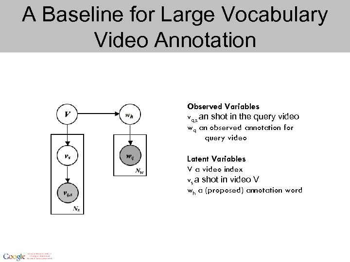
A Baseline for Large Vocabulary Video Annotation Observed Variables vq, s an shot in the query video wq an observed annotation for query video Latent Variables V a video index vs a shot in video V wh a (proposed) annotation word

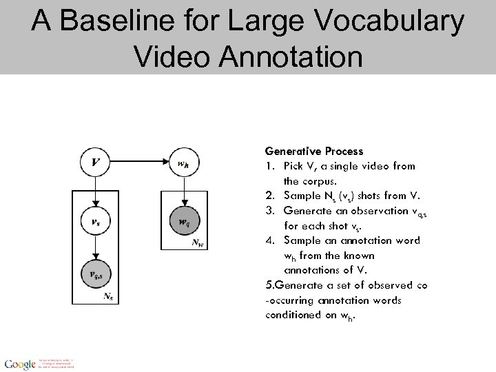
A Baseline for Large Vocabulary Video Annotation Generative Process 1. Pick V, a single video from the corpus. 2. Sample Ns (vs) shots from V. 3. Generate an observation vq, s for each shot vs. 4. Sample an annotation word wh from the known annotations of V. 5. Generate a set of observed co -occurring annotation words conditioned on wh.

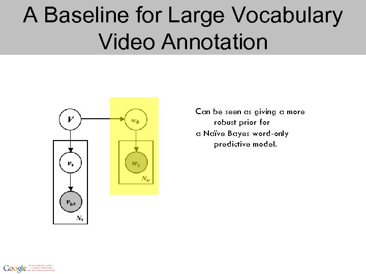
A Baseline for Large Vocabulary Video Annotation Can be seen as giving a more robust prior for a Naïve Bayes word-only predictive model.

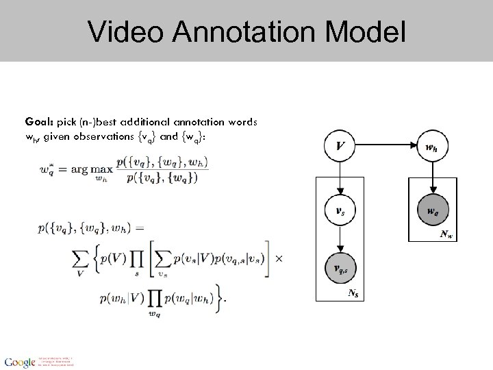
Video Annotation Model Goal: pick (n-)best additional annotation words wh, given observations {vq} and {wq}:

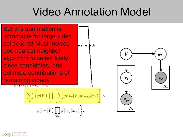
Video Annotation Model But this summation is intractable for large video collections! Must instead Goal: pick (n-)best additional annotation words w given observations {vq} and useh, nearest neighbor {wq}: algorithm to select likely close candidates, and estimate contributions of remaining videos.

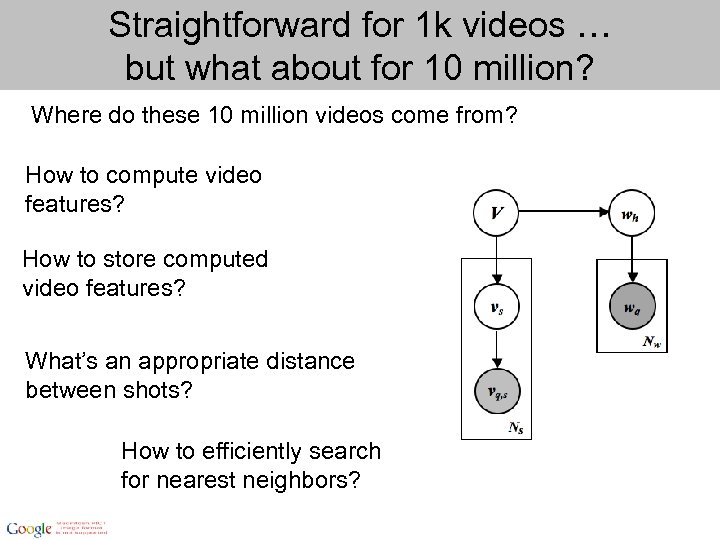
Straightforward for 1 k videos … but what about for 10 million? Where do these 10 million videos come from? How to compute video features? How to store computed video features? What’s an appropriate distance between shots? How to efficiently search for nearest neighbors?

Outline • • Probabilistic Model for Video Annotation You. Tube users Data centers System software infrastructure – Google File System – Map. Reduce – Bigtable • Machine-learning, computer vision – Distributed Spill Trees – Image Annotation • Preliminary experimental results

You. Tube People are watching hundreds of millions of videos a day on You. Tube and uploading hundreds of thousands of videos daily. Every minute, ten hours of video is uploaded to You. Tube.

Data-Centers (1) Machines are typically dual-processor x 86 processors running Linux, with 2 -4 GB of memory per machine. (2) Commodity networking hardware is used - typically either 100 megabits/second or 1 gigabit/second at the machine level, but averaging considerably less in overall bisection bandwidth. (3) A cluster consists of hundreds or thousands of machines, and therefore machine failures are common. (4) Storage is provided by inexpensive IDE disks attached directly to individual machines. Basic underlying hardware assumptions: Components are unreliable and failures are the norm not the exception.

and by the way … they’re Green! Efficient energy conversion from outlet to computing components Efficient energy management: 96% industry standard energy overhead, 21% at Google Recycle & Reuse electronic components Water cooling for heat management

Outline • • Probabilistic Model for Video Annotation You. Tube users Data centers System software infrastructure – Google File System – Map. Reduce – Bigtable • Machine-learning, computer vision – Distributed Spill Trees – Image Annotation • Preliminary experimental results

Google File System [Ghemawat, Gobioff, Leung SOSP 2003] Basic assumptions 1. Built on top of unreliable components 2. Extremely large files 3. Reading: either large streaming reads, or small random reads 4. Writing: primarily streaming appends 5. High sustained bandwidth more important than low latency

Google File System [Ghemawat, Gobioff, Leung SOSP 2003] Basic assumptions 1. Built on top of unreliable components 2. Extremely large files 3. Reading: either large streaming reads, or small random reads 4. Writing: primarily streaming appends 5. High sustained bandwidth more important than low latency For large-scale machine learning, this set of requirements is a pretty good fit!

Map. Reduce [Dean, Ghemawat, OSDI 2004] Goals • Large-scale data processing • Want to distribute across hundreds/thousands of machines • With an easy programming model, that can be applied to ad-hoc tasks Provides • Automatic parallelization and distribution • Fault-tolerance • I/O scheduling • Status and monitoring

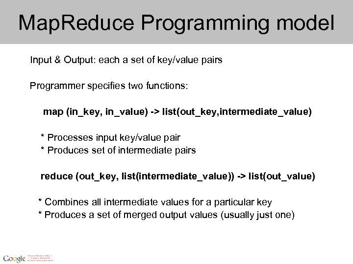
Map. Reduce Programming model Input & Output: each a set of key/value pairs Programmer specifies two functions: map (in_key, in_value) -> list(out_key, intermediate_value) * Processes input key/value pair * Produces set of intermediate pairs reduce (out_key, list(intermediate_value)) -> list(out_value) * Combines all intermediate values for a particular key * Produces a set of merged output values (usually just one)

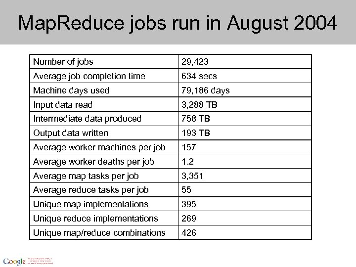
Map. Reduce jobs run in August 2004 Number of jobs 29, 423 Average job completion time 634 secs Machine days used 79, 186 days Input data read 3, 288 TB Intermediate data produced 758 TB Output data written 193 TB Average worker machines per job 157 Average worker deaths per job 1. 2 Average map tasks per job 3, 351 Average reduce tasks per job 55 Unique map implementations 395 Unique reduce implementations 269 Unique map/reduce combinations 426

Bigtable [Chang et al. OSDI 2006] • Distributed storage system: designed to scale to petabytes of data, across thousands of machines • Adaptable: handles throughput-oriented batch processing and latency-sensitive data serving to end-users Built on top of: Chubby [Burrows OSDI 2006] (distributed lock service) Google File System

Outline • • Probabilistic Model for Video Annotation You. Tube users Data centers System software infrastructure – Google File System – Map. Reduce – Bigtable • Machine-learning, computer vision – Distributed Spill Trees – Image Annotation • Preliminary experimental results

k-Nearest Neighbor Task: given a training set of instances, given a new query instance, find the k-nearest instances in the collection. These k-nearest instances can then be used to perform classification or regression as desired. Since it’s a non-parametric method, with more data, the method requires more data storage, and performing classification/regression for new instances takes increasing time. Have to reduce from a linear time. Metric Trees Spill Trees

Constructing a Metric Tree [Preperata and Shamos 1985]

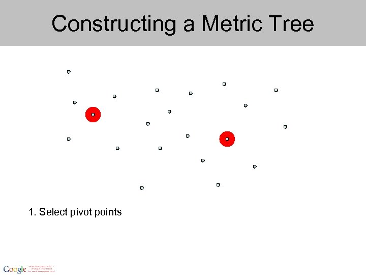
Constructing a Metric Tree 1. Select pivot points

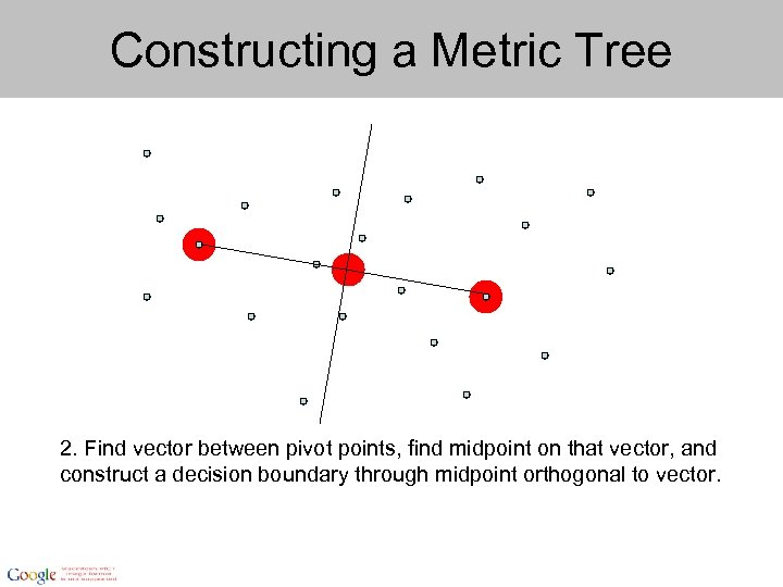
Constructing a Metric Tree 2. Find vector between pivot points, find midpoint on that vector, and construct a decision boundary through midpoint orthogonal to vector.

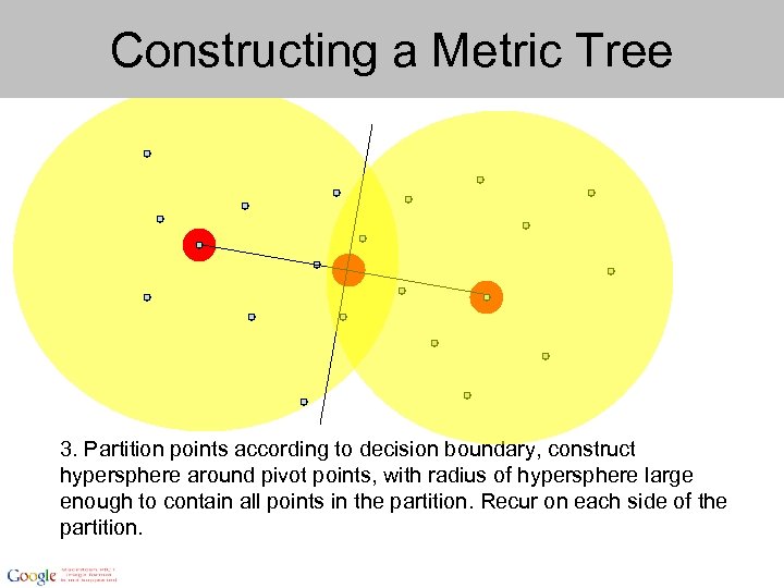
Constructing a Metric Tree 3. Partition points according to decision boundary, construct hypersphere around pivot points, with radius of hypersphere large enough to contain all points in the partition. Recur on each side of the partition.

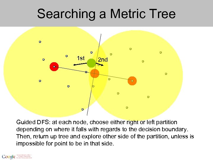
Searching a Metric Tree 1 st 2 nd Guided DFS: at each node, choose either right or left partition depending on where it falls with regards to the decision boundary. Then, return up tree and explore other side of the partition, unless is impossible for point to be in that side.

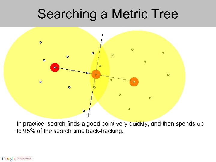
Searching a Metric Tree In practice, search finds a good point very quickly, and then spends up to 95% of the search time back-tracking.

Constructing a Spill Tree [Liu, Moore, Gray Yang NIPS 2004 ] 1. Like metric tree, construct first decision boundary. Next, construct planes parallel to decision boundary and distance away.

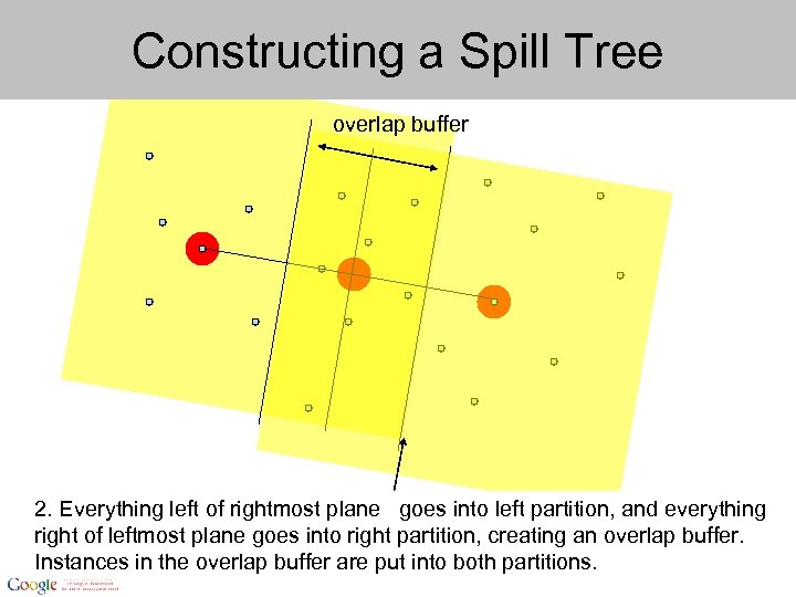
Constructing a Spill Tree overlap buffer 2. Everything left of rightmost plane goes into left partition, and everything right of leftmost plane goes into right partition, creating an overlap buffer. Instances in the overlap buffer are put into both partitions.

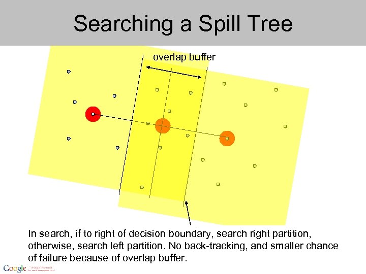
Searching a Spill Tree overlap buffer In search, if to right of decision boundary, search right partition, otherwise, search left partition. No back-tracking, and smaller chance of failure because of overlap buffer.

Distributed Spill Trees [Liu, Rosenberg, Rowley IEEE WACV 2007 ] If each instance is 416 bytes (104 dimensions), in one 4 GB machine, you can store 8 million instances (in memory). Goal of [Liu et al. 2007] project was to operate over 1 billion instances, so around 100 machines would be needed. A Distributed Spill Tree is required.

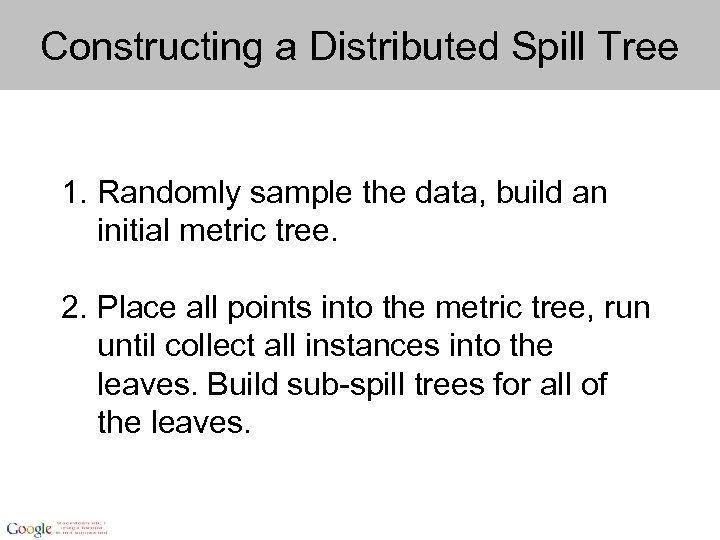
Constructing a Distributed Spill Tree 1. Randomly sample the data, build an initial metric tree. 2. Place all points into the metric tree, run until collect all instances into the leaves. Build sub-spill trees for all of the leaves.

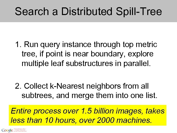
Search a Distributed Spill-Tree 1. Run query instance through top metric tree, if point is near boundary, explore multiple leaf substructures in parallel. 2. Collect k-Nearest neighbors from all subtrees, and merge them into one list. Entire process over 1. 5 billion images, takes less than 10 hours, over 2000 machines.

Outline • • Probabilistic Model for Video Annotation You. Tube users Data centers System software infrastructure – Google File System – Map. Reduce – Bigtable • Machine-learning, computer vision – Distributed Spill Trees – Image Annotation • Preliminary experimental results

Image Annotation [Makadia, Pavlovic, Kumar, ECCV 2008] Given an input image, the goal of automatic image annotation is to assign a few relevant text keywords to the image that reflect its visual content. This problem is of great interest as it allows one to index and retrieve large image collections using current text-based search engines.

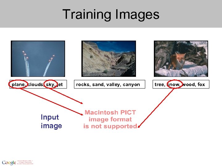
Training Images plane, clouds, sky, jet Input image rocks, sand, valley, canyon tree, snow, wood, fox

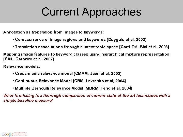
Current Approaches Annotation as translation from images to keywords: • Co-occurrence of image regions and keywords [Duygulu et al, 2002] • Translation associations through a latent topic space [Corr. LDA, Blei et al, 2003] Mapping image features to keyword classes using hierarchical mixture representation [SML, Carneiro et al, 2007] Relevance models: • Cross-media relevance model [CMRM, Jeon et al, 2003] • Continuous Relevance Model [CRM, Lavrenko et al, 2004] • Multiple Bernoulli Relevance Model [MBRM, Feng et al, 2004] What is missing is a thorough comparison of current state-of-the-art techniques with a simple baseline measure!

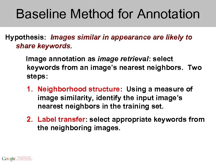
Baseline Method for Annotation Hypothesis: Images similar in appearance are likely to share keywords. Image annotation as image retrieval: select keywords from an image’s nearest neighbors. Two steps: 1. Neighborhood structure: Using a measure of image similarity, identify the input image’s nearest neighbors in the training set. 2. Label transfer: select appropriate keywords from the neighboring images.

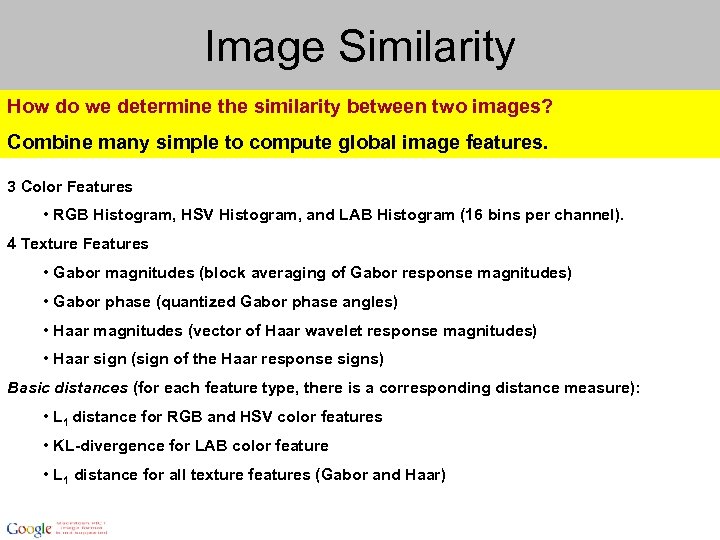
Image Similarity How do we determine the similarity between two images? Combine many simple to compute global image features. 3 Color Features • RGB Histogram, HSV Histogram, and LAB Histogram (16 bins per channel). 4 Texture Features • Gabor magnitudes (block averaging of Gabor response magnitudes) • Gabor phase (quantized Gabor phase angles) • Haar magnitudes (vector of Haar wavelet response magnitudes) • Haar sign (sign of the Haar response signs) Basic distances (for each feature type, there is a corresponding distance measure): • L 1 distance for RGB and HSV color features • KL-divergence for LAB color feature • L 1 distance for all texture features (Gabor and Haar)

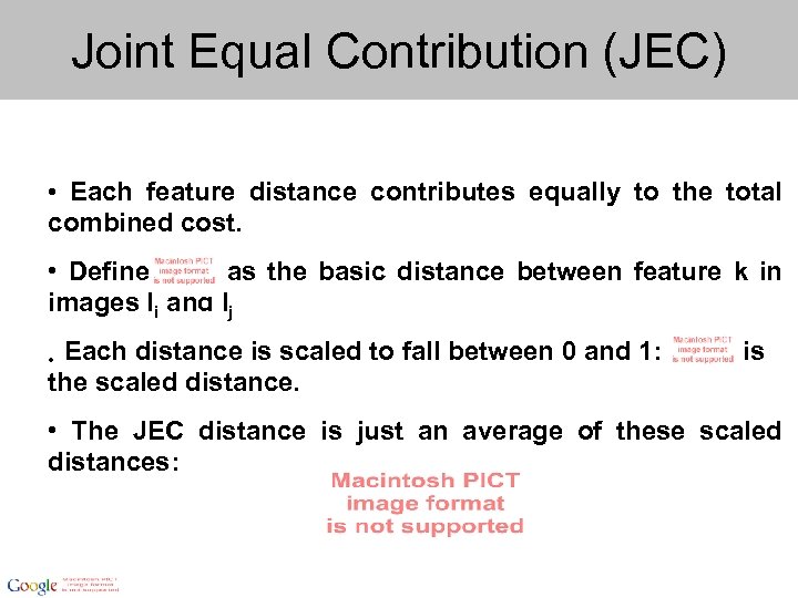
Joint Equal Contribution (JEC) • Each feature distance contributes equally to the total combined cost. • Define as the basic distance between feature k in images Ii and Ij Each distance is scaled to fall between 0 and 1: the scaled distance. • is • The JEC distance is just an average of these scaled distances:

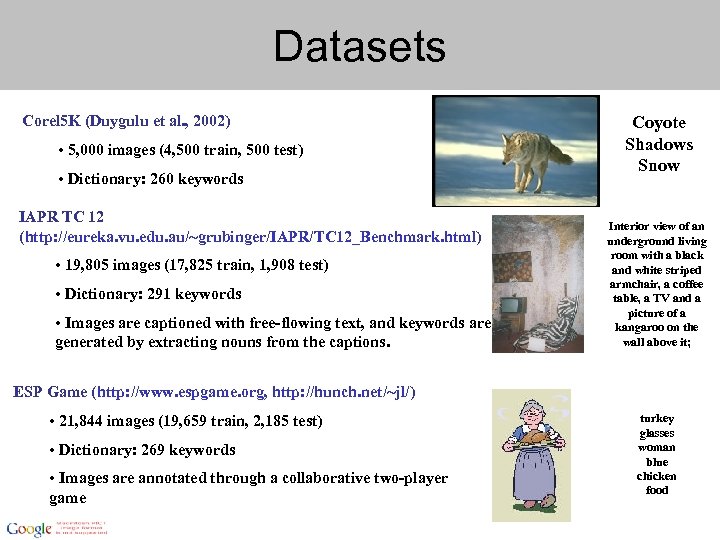
Datasets Corel 5 K (Duygulu et al. , 2002) • 5, 000 images (4, 500 train, 500 test) • Dictionary: 260 keywords IAPR TC 12 (http: //eureka. vu. edu. au/~grubinger/IAPR/TC 12_Benchmark. html) • 19, 805 images (17, 825 train, 1, 908 test) • Dictionary: 291 keywords • Images are captioned with free-flowing text, and keywords are generated by extracting nouns from the captions. Coyote Shadows Snow Interior view of an underground living room with a black and white striped armchair, a coffee table, a TV and a picture of a kangaroo on the wall above it; ESP Game (http: //www. espgame. org, http: //hunch. net/~jl/) • 21, 844 images (19, 659 train, 2, 185 test) • Dictionary: 269 keywords • Images are annotated through a collaborative two-player game turkey glasses woman blue chicken food

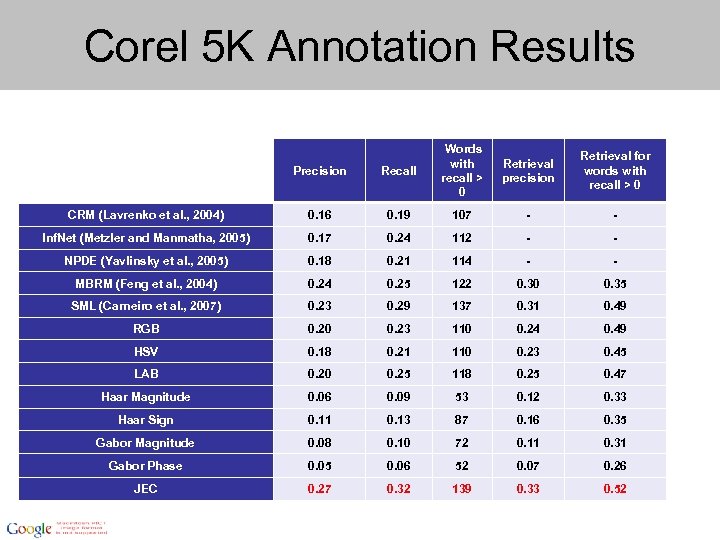
Corel 5 K Annotation Results Precision Recall Words with recall > 0 CRM (Lavrenko et al. , 2004) 0. 16 0. 19 107 - - Inf. Net (Metzler and Manmatha, 2005) 0. 17 0. 24 112 - - NPDE (Yavlinsky et al. , 2005) 0. 18 0. 21 114 - - MBRM (Feng et al. , 2004) 0. 24 0. 25 122 0. 30 0. 35 SML (Carneiro et al. , 2007) 0. 23 0. 29 137 0. 31 0. 49 RGB 0. 20 0. 23 110 0. 24 0. 49 HSV 0. 18 0. 21 110 0. 23 0. 45 LAB 0. 20 0. 25 118 0. 25 0. 47 Haar Magnitude 0. 06 0. 09 53 0. 12 0. 33 Haar Sign 0. 11 0. 13 87 0. 16 0. 35 Gabor Magnitude 0. 08 0. 10 72 0. 11 0. 31 Gabor Phase 0. 05 0. 06 52 0. 07 0. 26 JEC 0. 27 0. 32 139 0. 33 0. 52 Retrieval precision Retrieval for words with recall > 0

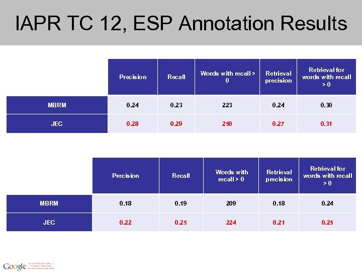
IAPR TC 12, ESP Annotation Results Retrieval precision Retrieval for words with recall >0 Precision Recall Words with recall > 0 MBRM 0. 24 0. 23 223 0. 24 0. 30 JEC 0. 28 0. 29 250 0. 27 0. 31 Retrieval precision Retrieval for words with recall >0 Precision Recall Words with recall > 0 MBRM 0. 18 0. 19 209 0. 18 0. 24 JEC 0. 22 0. 25 224 0. 21 0. 25

Outline • • Probabilistic Model for Video Annotation You. Tube users Data centers System software infrastructure – Google File System – Map. Reduce – Bigtable • Machine-learning, computer vision – Distributed Spill Trees – Image Annotation • Preliminary experimental results

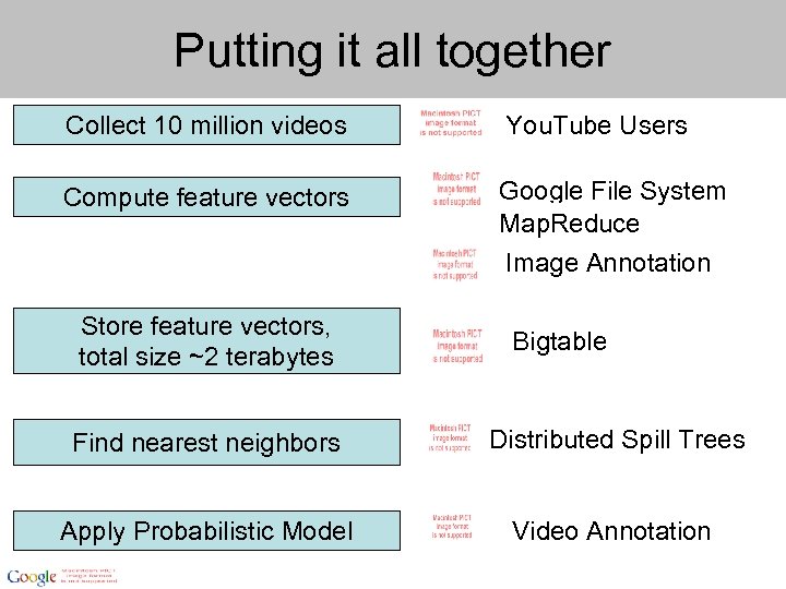
Putting it all together Collect 10 million videos You. Tube Users Compute feature vectors Google File System Map. Reduce Image Annotation Store feature vectors, total size ~2 terabytes Bigtable Find nearest neighbors Distributed Spill Trees Apply Probabilistic Model Video Annotation

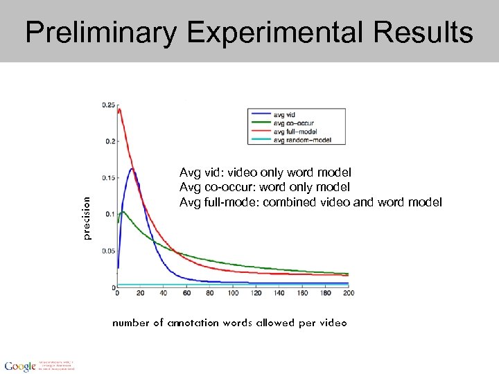
precision Preliminary Experimental Results Avg vid: video only word model Avg co-occur: word only model Avg full-mode: combined video and word model number of annotation words allowed per video

Conclusion • Probabilistic Video Annotation Model that proposes new annotations by integrated existing annotations and information from videon content • Google user/hardware/software ecology can enable rapid progress on research and suggest new areas for work.

Social Next Ice-cream! Googlers on hand to answer questions. Leslie Yeh Johnson Vitaliy Lvin Lijuan Cai