875 -8 ppt 8 Applied GE modeling of

875 -8. ppt 8 Applied GE modeling of economy & environment 1. Rationales 2. Basics of applied GE models 3. Incorporating environmental issues 4. An application Main source: OEE Ch. 5. Additional: Shoven & Whalley, JEL 1984; Ginsburgh & Keyzer, Structure of applied general eq. models (MIT Press, 1997); Coxhead, World Development 28(1), 2000.

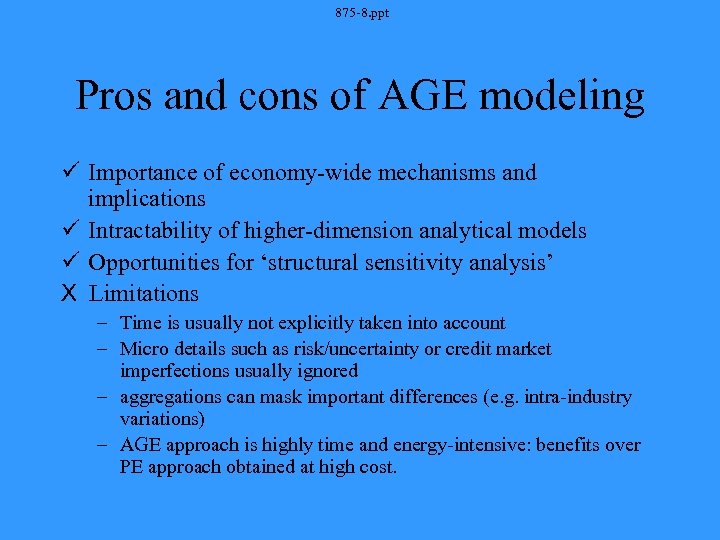875 -8. ppt Pros and cons of AGE modeling ü Importance of economy-wide mechanisms and implications ü Intractability of higher-dimension analytical models ü Opportunities for ‘structural sensitivity analysis’ X Limitations – Time is usually not explicitly taken into account – Micro details such as risk/uncertainty or credit market imperfections usually ignored – aggregations can mask important differences (e. g. intra-industry variations) – AGE approach is highly time and energy-intensive: benefits over PE approach obtained at high cost.

875 -8. ppt Overview of AGE models • Describe Walrasian equilibria in fairly detailed manner--sufficient to support policy claims – Too large to be solved analytically; must use numerical solutions instead – But structure and results depend on same theoretical foundations • Advantages and disadvantages of size.

875 -8. ppt An N-good, F-factor economy • General structure • Equilibrium conditions • Closure rules and decisions

875 -8. ppt Variables in the basic model 5

875 -8. ppt 6

875 -8. ppt 7

875 -8. ppt Closure • No. of equations must match endog. vars. – In (5. 1)-(5. 8): 4 N + FN + M + 1 eqns. – But we have 5 N + 2 F + FN + 2 variables. – Must choose N - M + F + 1 exog. vars • Declare V exog; (N - M) elements of P, and . • Now (5. 1)-(5. 8) solves for Y, W, R, X, D, S and U as endogenous variables. – Endogenous: income, factor prices, quantities produced and demanded, trade, and utility. – Exogenous: factor endowments, traded goods’ prices and a numeraire price.

875 -8. ppt Closure rules and decisions • Other closures are possible – ‘Neoclassical’ closure has all domestic prices flexible – Alternatives: e. g. fix wages, allow unemployment in labor market. • These choices reflect our beliefs or observations about the real world.

875 -8. ppt Other features • Can add in: – Intermediate inputs – Products distinguished by source (domestic, imported) – Different kinds of labor – Many sources of final demand – Trade and transport ‘margins’ – Tariffs, taxes, and other policies … etc.

875 -8. ppt Solving the model: the ‘Johansen’ AGE structure • First-order approximations to changes in variable values • Models solved in proportional (percentage) changes of variables, or ‘hat calculus’. • Advantages: – Models are linear in variables – Parameter values are intuitive and accessible (shares from SAM, elasticities from other sources) – Simulation results are additive in separate shocks

875 -8. ppt Features of Johansen models • Parameter values are shares and elasticities • Quick checks: – Homogeneity & ‘balance’ of underlying data base. • Solution is by matrix inversion – Entire model is a system of linear equations • Examples of Johansen-style models: – ORANI (Australian economy) – GTAP (international agricultural trade) – Models in OEE, Ch. 6– 8

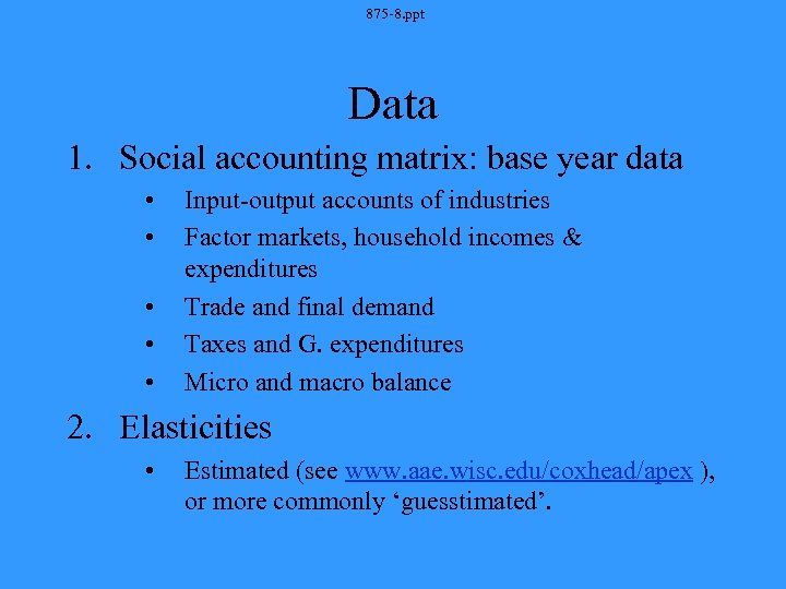875 -8. ppt Data 1. Social accounting matrix: base year data • • • Input-output accounts of industries Factor markets, household incomes & expenditures Trade and final demand Taxes and G. expenditures Micro and macro balance 2. Elasticities • Estimated (see www. aae. wisc. edu/coxhead/apex ), or more commonly ‘guesstimated’.

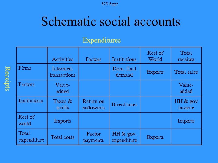875 -8. ppt Schematic social accounts Expenditures Activities Receipts Firms Factors Institutions Rest of world Total expenditure Factors Intermed. transactions Institutions Dom. final demand Rest of World Total receipts Exports Total sales Valueadded Taxes & tariffs Valueadded Return on endowmts HH & gov income Direct taxes Imports Total costs Imports Factor payments HH & gov. expenditure Exports

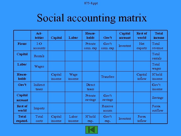875 -8. ppt Social accounting matrix Activities Firms Capital Labor I-O accounts Gov’t cons. exp Capital account Rest of world Total income Investmt Net exports Total revenue Rentals Total rentals Wages Total wages Households Gov’t Labor Gov’t Private cons. exp Capital Households Capital income Wage income Indirect taxes Direct taxes Capital account Private savings Rest of world Total costs H’hold income Gov’t income Capital income Labor income H’hold exp. Gov’t savings Savings Reserve accum Imports Total expend. Capital inflow Transfers Forex outflow Gov’t exp. Investmt Forex inflow

875 -8. ppt ‘Standard’ national accounts ignore environment • Assumptions: – Property rights on resources – No externalities – No non-marketed amenity values

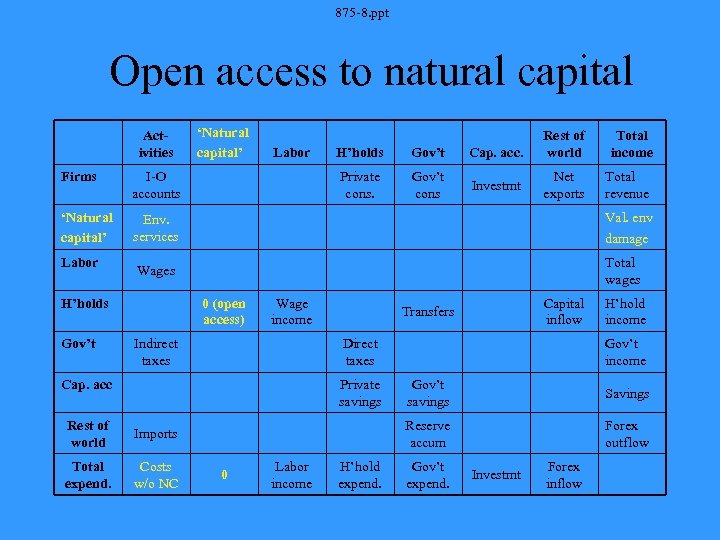875 -8. ppt Open access to natural capital Activities ‘Natural capital’ Labor H’holds Gov’t Cap. acc. Private cons. Gov’t cons Investmt Rest of world Total income Net exports Total revenue Firms I-O accounts ‘Natural capital’ Env. services Val. env damage Wages Total wages Labor H’holds Gov’t 0 (open access) Wage income Indirect taxes Direct taxes Cap. acc Private savings Rest of world Costs w/o NC H’hold income Gov’t income 0 Labor income H’hold expend. Gov’t savings Savings Reserve accum Imports Total expend. Capital inflow Transfers Forex outflow Gov’t expend. Investmt Forex inflow

875 -8. ppt Addressing env. damages and natural resource depletion • Pigovian taxes (Bovenberg & Goulder, AER 1996) • Private purchase of abatement services • Public provision of abatement or clean-up services • Quotas or limits on resource use or emissions (command & control)

875 -8. ppt Environmental analysis in GE • Most AGE models constructed for more general analytical purposes: environmental structure is added later • Given uncertainty about env. variables and valuations this may be appropriate! • Industrial emissions: ‘side calculations’ • Natural resource degradation • Questions about institutions.

875 -8. ppt Deforestation & land degradation • Commercial and non-comm’l deforestation: does timber have market value? – Non-comm’l deforestation is driven by search for land, and responds to changes in the marginal valuation of land in agricultural production. . . – … although institutional setting also matters

875 -8. ppt Land degradation • Hard to measure, and problems of aggregation. • Can use information on erosion rates by crop, together with land use data, to build ‘baseline’ data set. – Then erosion changes can be inferred from changes in land use • Production externalities: technical ‘regress’.

875 -8. ppt Institutional issues 1. Trees may be cut (or planted) to establish property rights over land. In open access forests (non-commercial), opportunity cost of forest is set by ag. land values and clearing costs. In commercial forestry, timber harvesting/replanting also depends on property rights. 2. 3. • Will an increase in timber prices promote or retard tree-felling in aggregate? Depends on property rights.

875 -8. ppt ‘Structural sensitivity analysis’ • Alter assumptions about market clearing • Alter assumptions about property rights • Alter assumptions about macroeconomic closure – e. g. Adjustment to equilibrium through domestic tax system vs. adjustments through accommodating international capital flows.