 7 TOPICS FOR FURTHER STUDY
 The Theory of Consumer Choice Copyright© 2004 South-Western 21
 • The theory of consumer choice addresses the following questions: • Do all demand curves slope downward? • How do wages affect labor supply? • How do interest rates affect household saving? Copyright© 2004 South-Western
 THE BUDGET CONSTRAINT: WHAT THE CONSUMER CAN AFFORD • The budget constraint depicts the limit on the consumption “bundles” that a consumer can afford. • People consume less than they desire because their spending is constrained, or limited, by their income. Copyright© 2004 South-Western
 THE BUDGET CONSTRAINT: WHAT THE CONSUMER CAN AFFORD • The budget constraint shows the various combinations of goods the consumer can afford given his or her income and the prices of the two goods. Copyright© 2004 South-Western
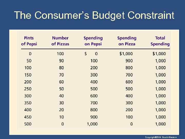 The Consumer’s Budget Constraint Copyright© 2004 South-Western
 THE BUDGET CONSTRAINT: WHAT THE CONSUMER CAN AFFORD • The Consumer’s Budget Constraint • Any point on the budget constraint line indicates the consumer’s combination or tradeoff between two goods. • For example, if the consumer buys no pizzas, he can afford 500 pints of Pepsi (point B). If he buys no Pepsi, he can afford 100 pizzas (point A). Copyright© 2004 South-Western
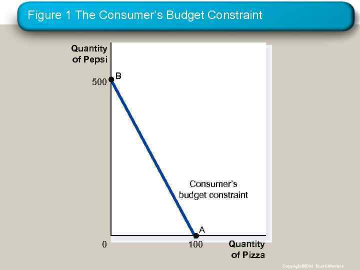 Figure 1 The Consumer’s Budget Constraint Quantity of Pepsi 500 B Consumer’s budget constraint A 0 100 Quantity of Pizza Copyright© 2004 South-Western
 THE BUDGET CONSTRAINT: WHAT THE CONSUMER CAN AFFORD • The Consumer’s Budget Constraint • Alternately, the consumer can buy 50 pizzas and 250 pints of Pepsi. Copyright© 2004 South-Western
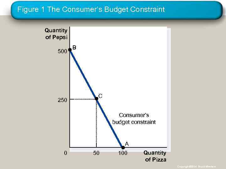 Figure 1 The Consumer’s Budget Constraint Quantity of Pepsi 500 250 B C Consumer’s budget constraint A 0 50 100 Quantity of Pizza Copyright© 2004 South-Western
 THE BUDGET CONSTRAINT: WHAT THE CONSUMER CAN AFFORD • The slope of the budget constraint line equals the relative price of the two goods, that is, the price of one good compared to the price of the other. • It measures the rate at which the consumer can trade one good for the other. Copyright© 2004 South-Western
 PREFERENCES: WHAT THE CONSUMER WANTS • A consumer’s preference among consumption bundles may be illustrated with indifference curves. Copyright© 2004 South-Western
 Representing Preferences with Indifference Curves • An indifference curve is a curve that shows consumption bundles that give the consumer the same level of satisfaction. Copyright© 2004 South-Western
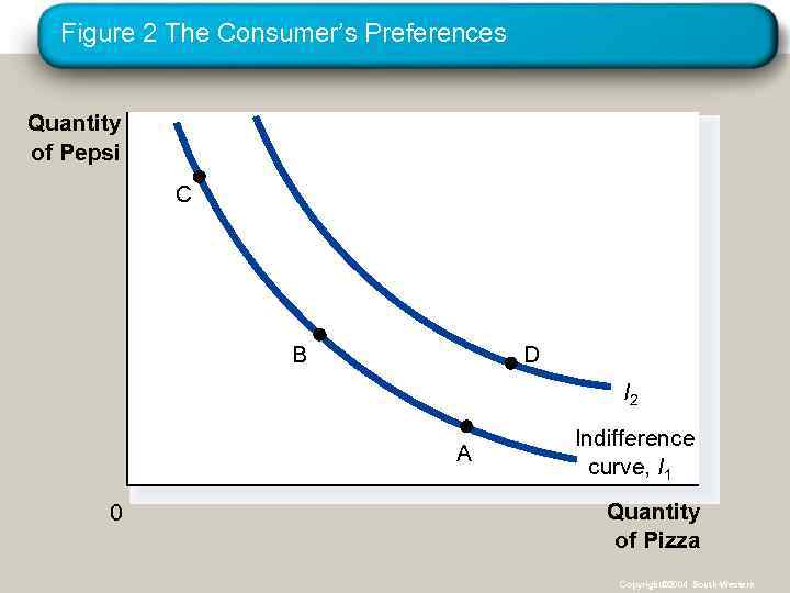 Figure 2 The Consumer’s Preferences Quantity of Pepsi C B D I 2 A 0 Indifference curve, I 1 Quantity of Pizza Copyright© 2004 South-Western
 Representing Preferences with Indifference Curves • The Consumer’s Preferences • The consumer is indifferent, or equally happy, with the combinations shown at points A, B, and C because they are all on the same curve. • The Marginal Rate of Substitution • The slope at any point on an indifference curve is the marginal rate of substitution. • It is the rate at which a consumer is willing to trade one good for another. • It is the amount of one good that a consumer requires as compensation to give up one unit of the other good. Copyright© 2004 South-Western
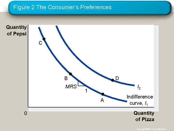 Figure 2 The Consumer’s Preferences Quantity of Pepsi C B MRS D I 2 1 A 0 Indifference curve, I 1 Quantity of Pizza Copyright© 2004 South-Western
 Four Properties of Indifference Curves • Higher indifference curves are preferred to lower ones. • Indifference curves are downward sloping. • Indifference curves do not cross. • Indifference curves are bowed inward. Copyright© 2004 South-Western
 Four Properties of Indifference Curves • Property 1: Higher indifference curves are preferred to lower ones. • Consumers usually prefer more of something to less of it. • Higher indifference curves represent larger quantities of goods than do lower indifference curves. Copyright© 2004 South-Western
 Figure 2 The Consumer’s Preferences Quantity of Pepsi C B D I 2 A 0 Indifference curve, I 1 Quantity of Pizza Copyright© 2004 South-Western
 Four Properties of Indifference Curves • Property 2: Indifference curves are downward sloping. • A consumer is willing to give up one good only if he or she gets more of the other good in order to remain equally happy. • If the quantity of one good is reduced, the quantity of the other good must increase. • For this reason, most indifference curves slope downward. Copyright© 2004 South-Western
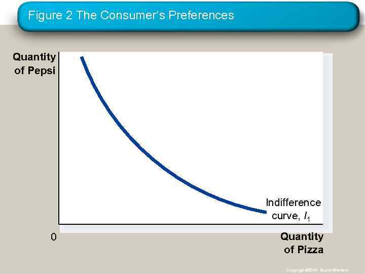 Figure 2 The Consumer’s Preferences Quantity of Pepsi Indifference curve, I 1 0 Quantity of Pizza Copyright© 2004 South-Western
 Four Properties of Indifference Curves • Property 3: Indifference curves do not cross. • Points A and B should make the consumer equally happy. • Points B and C should make the consumer equally happy. • This implies that A and C would make the consumer equally happy. • But C has more of both goods compared to A. Copyright© 2004 South-Western
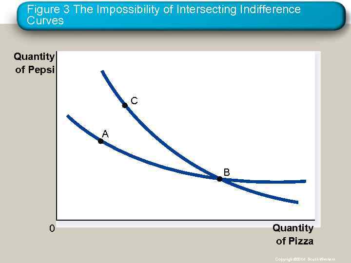 Figure 3 The Impossibility of Intersecting Indifference Curves Quantity of Pepsi C A B 0 Quantity of Pizza Copyright© 2004 South-Western
 Four Properties of Indifference Curves • Property 4: Indifference curves are bowed inward. • People are more willing to trade away goods that they have in abundance and less willing to trade away goods of which they have little. • These differences in a consumer’s marginal substitution rates cause his or her indifference curve to bow inward. Copyright© 2004 South-Western
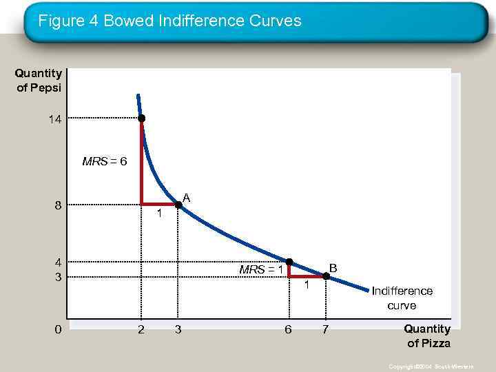 Figure 4 Bowed Indifference Curves Quantity of Pepsi 14 MRS = 6 A 8 1 4 3 0 B MRS = 1 1 2 3 6 Indifference curve 7 Quantity of Pizza Copyright© 2004 South-Western
 Two Extreme Examples of Indifference Curves • Perfect substitutes • Perfect complements Copyright© 2004 South-Western
 Two Extreme Examples of Indifference Curves • Perfect Substitutes • Two goods with straight-line indifference curves are perfect substitutes. • The marginal rate of substitution is a fixed number. Copyright© 2004 South-Western
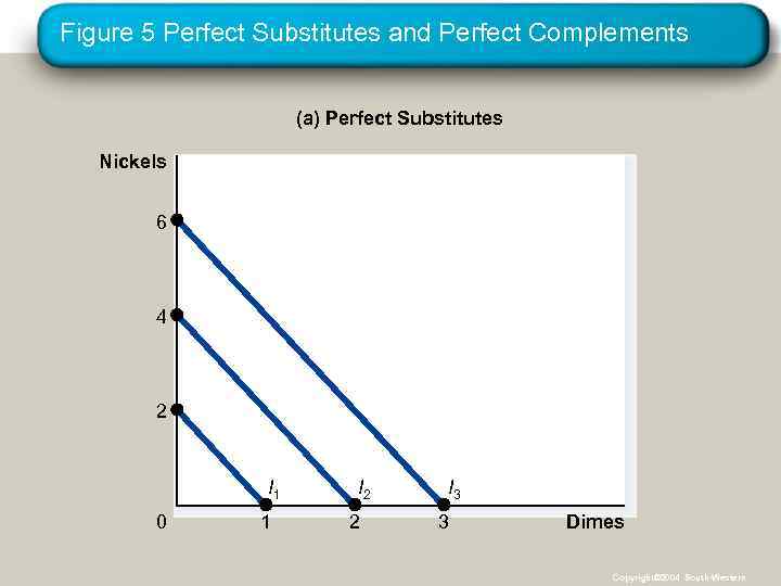 Figure 5 Perfect Substitutes and Perfect Complements (a) Perfect Substitutes Nickels 6 4 2 I 1 0 1 I 2 2 I 3 3 Dimes Copyright© 2004 South-Western
 Two Extreme Examples of Indifference Curves • Perfect Complements • Two goods with right-angle indifference curves are perfect complements. Copyright© 2004 South-Western
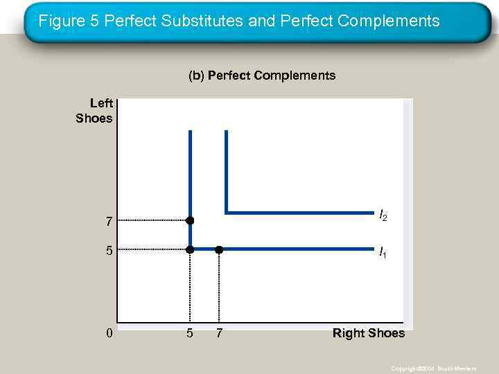 Figure 5 Perfect Substitutes and Perfect Complements (b) Perfect Complements Left Shoes 7 I 2 5 I 1 0 5 7 Right Shoes Copyright© 2004 South-Western
 OPTIMIZATION: WHAT THE CONSUMER CHOOSES • Consumers want to get the combination of goods on the highest possible indifference curve. • However, the consumer must also end up on or below his budget constraint. Copyright© 2004 South-Western
 The Consumer’s Optimal Choices • Combining the indifference curve and the budget constraint determines the consumer’s optimal choice. • Consumer optimum occurs at the point where the highest indifference curve and the budget constraint are tangent. Copyright© 2004 South-Western
 The Consumer’s Optimal Choice • The consumer chooses consumption of the two goods so that the marginal rate of substitution equals the relative price. Copyright© 2004 South-Western
 The Consumer’s Optimal Choice • At the consumer’s optimum, the consumer’s valuation of the two goods equals the market’s valuation. Copyright© 2004 South-Western
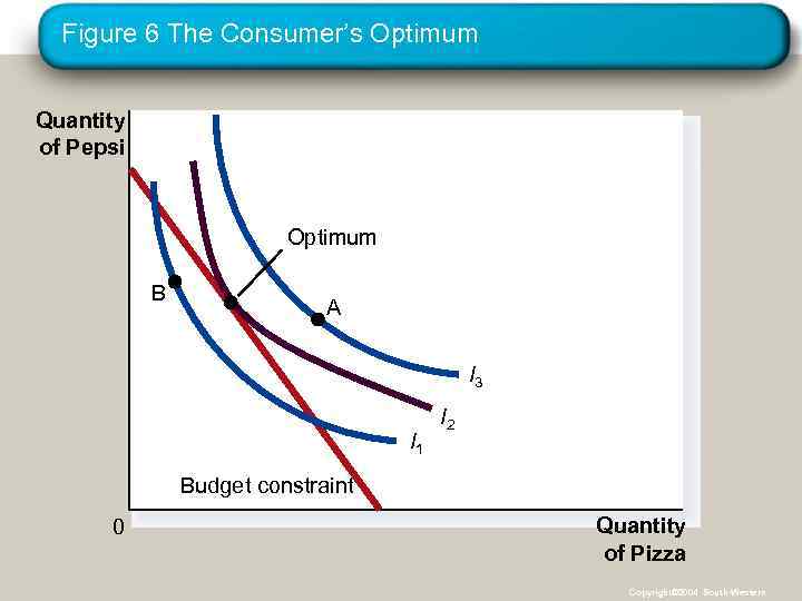 Figure 6 The Consumer’s Optimum Quantity of Pepsi Optimum B A I 3 I 1 I 2 Budget constraint 0 Quantity of Pizza Copyright© 2004 South-Western
 How Changes in Income Affect the Consumer’s Choices • An increase in income shifts the budget constraint outward. • The consumer is able to choose a better combination of goods on a higher indifference curve. Copyright© 2004 South-Western
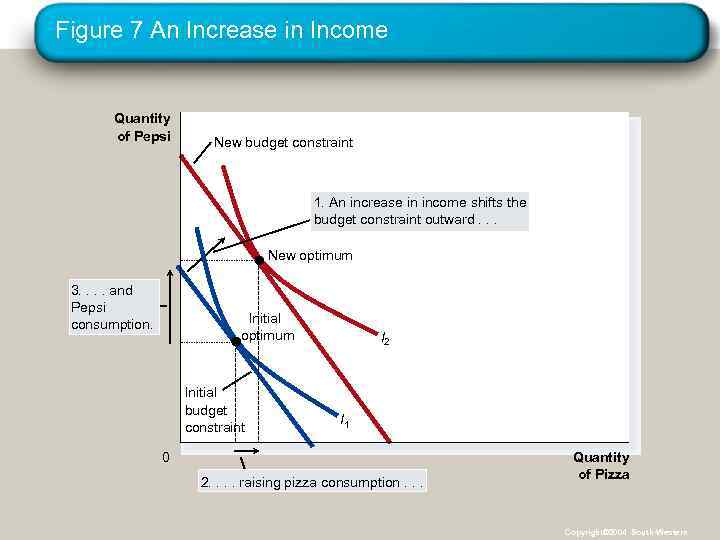 Figure 7 An Increase in Income Quantity of Pepsi New budget constraint 1. An increase in income shifts the budget constraint outward. . . New optimum 3. . and Pepsi consumption. Initial optimum Initial budget constraint I 2 I 1 0 2. . raising pizza consumption. . . Quantity of Pizza Copyright© 2004 South-Western
 How Changes in Income Affect the Consumer’s Choices • Normal versus Inferior Goods • If a consumer buys more of a good when his or her income rises, the good is called a normal good. • If a consumer buys less of a good when his or her income rises, the good is called an inferior good. Copyright© 2004 South-Western
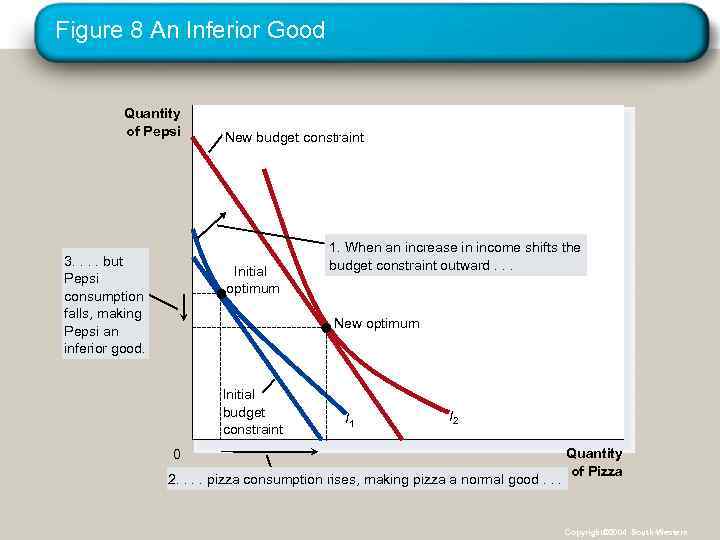 Figure 8 An Inferior Good Quantity of Pepsi 3. . but Pepsi consumption falls, making Pepsi an inferior good. New budget constraint Initial optimum 1. When an increase in income shifts the budget constraint outward. . . New optimum Initial budget constraint I 1 I 2 0 2. . pizza consumption rises, making pizza a normal good. . . Quantity of Pizza Copyright© 2004 South-Western
 How Changes in Prices Affect Consumer’s Choices • A fall in the price of any good rotates the budget constraint outward and changes the slope of the budget constraint. Copyright© 2004 South-Western
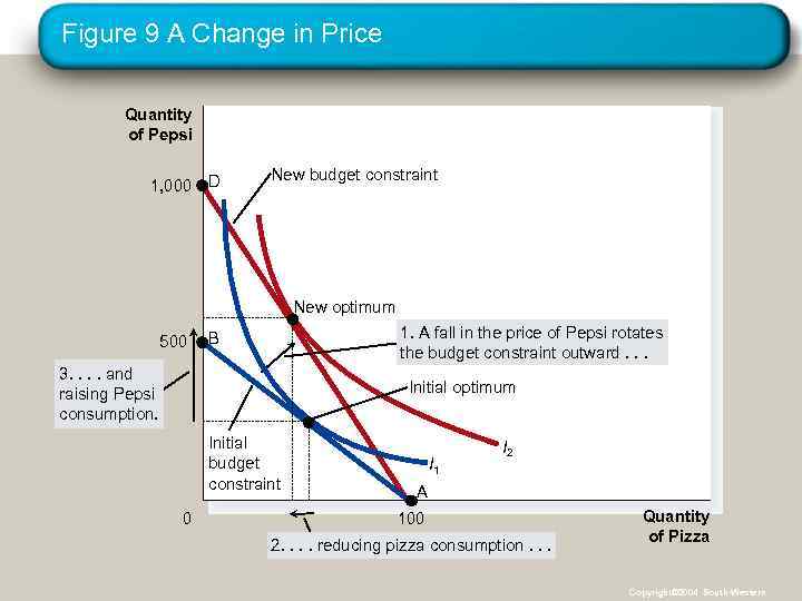 Figure 9 A Change in Price Quantity of Pepsi 1, 000 D New budget constraint New optimum 500 1. A fall in the price of Pepsi rotates the budget constraint outward. . . B 3. . and raising Pepsi consumption. Initial optimum Initial budget constraint 0 I 1 I 2 A 100 2. . reducing pizza consumption. . . Quantity of Pizza Copyright© 2004 South-Western
 Income and Substitution Effects • A price change has two effects on consumption. • An income effect • A substitution effect Copyright© 2004 South-Western
 Income and Substitution Effects • The Income Effect • The income effect is the change in consumption that results when a price change moves the consumer to a higher or lower indifference curve. • The Substitution Effect • The substitution effect is the change in consumption that results when a price change moves the consumer along an indifference curve to a point with a different marginal rate of substitution. Copyright© 2004 South-Western
 Income and Substitution Effects • A Change in Price: Substitution Effect • A price change first causes the consumer to move from one point on an indifference curve to another on the same curve. • Illustrated by movement from point A to point B. • A Change in Price: Income Effect • After moving from one point to another on the same curve, the consumer will move to another indifference curve. • Illustrated by movement from point B to point C. Copyright© 2004 South-Western
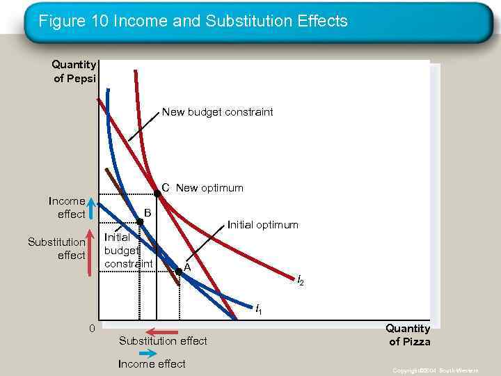 Figure 10 Income and Substitution Effects Quantity of Pepsi New budget constraint C New optimum Income effect B Substitution effect Initial budget constraint Initial optimum A I 2 I 1 0 Substitution effect Income effect Quantity of Pizza Copyright© 2004 South-Western
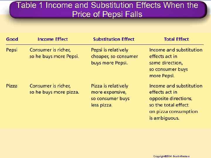 Table 1 Income and Substitution Effects When the Price of Pepsi Falls Copyright© 2004 South-Western
 Deriving the Demand Curve • A consumer’s demand curve can be viewed as a summary of the optimal decisions that arise from his or her budget constraint and indifference curves. Copyright© 2004 South-Western
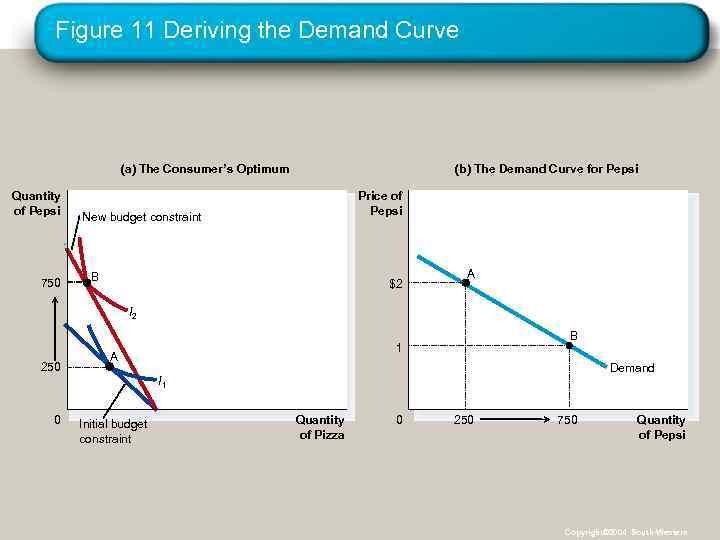 Figure 11 Deriving the Demand Curve (a) The Consumer’s Optimum Quantity of Pepsi 750 (b) The Demand Curve for Pepsi Price of Pepsi New budget constraint B $2 A I 2 250 B 1 A Demand I 1 0 Initial budget constraint Quantity of Pizza 0 250 750 Quantity of Pepsi Copyright© 2004 South-Western
 THREE APPLICATIONS • Do all demand curves slope downward? • Demand curves can sometimes slope upward. • This happens when a consumer buys more of a good when its price rises. • Giffen goods • Economists use the term Giffen good to describe a good that violates the law of demand. • Giffen goods are goods for which an increase in the price raises the quantity demanded. • The income effect dominates the substitution effect. • They have demand curves that slope upwards. Copyright© 2004 South-Western
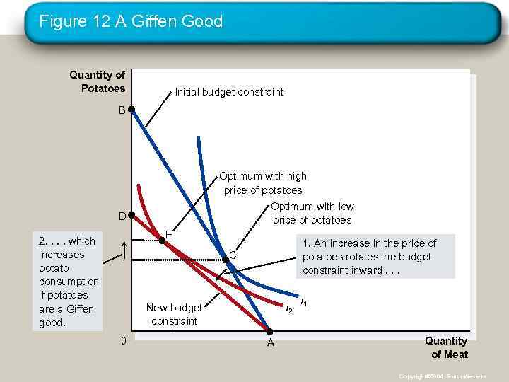 Figure 12 A Giffen Good Quantity of Potatoes Initial budget constraint B Optimum with high price of potatoes Optimum with low price of potatoes D E 2. . which increases potato consumption if potatoes are a Giffen good. 1. An increase in the price of potatoes rotates the budget constraint inward. . . C New budget constraint 0 I 2 A I 1 Quantity of Meat Copyright© 2004 South-Western
 THREE APPLICATIONS • How do wages affect labor supply? • If the substitution effect is greater than the income effect for the worker, he or she works more. • If income effect is greater than the substitution effect, he or she works less. Copyright© 2004 South-Western
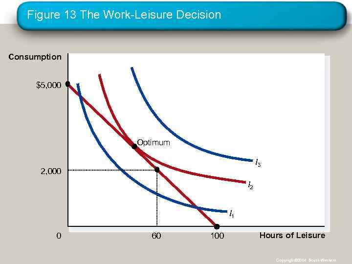 Figure 13 The Work-Leisure Decision Consumption $5, 000 Optimum I 3 2, 000 I 2 I 1 0 60 100 Hours of Leisure Copyright© 2004 South-Western
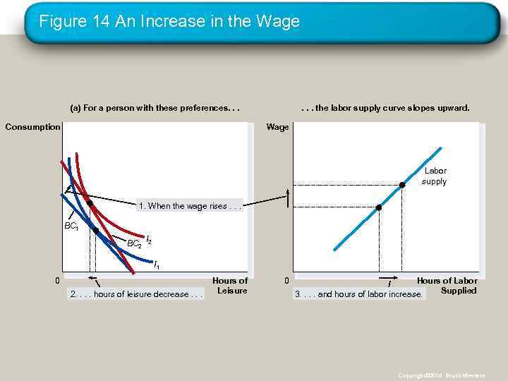 Figure 14 An Increase in the Wage (a) For a person with these preferences. . . Consumption . . . the labor supply curve slopes upward. Wage Labor supply 1. When the wage rises. . . BC 1 BC 2 I 1 0 2. . hours of leisure decrease. . . Hours of Leisure 0 Hours of Labor Supplied 3. . and hours of labor increase. Copyright© 2004 South-Western
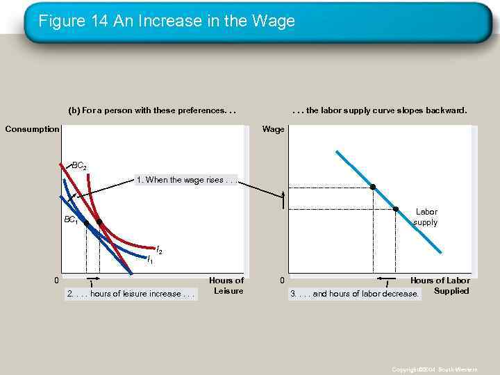 Figure 14 An Increase in the Wage (b) For a person with these preferences. . . Consumption . . . the labor supply curve slopes backward. Wage BC 2 1. When the wage rises. . . Labor supply BC 1 I 2 0 2. . hours of leisure increase. . . Hours of Leisure 0 Hours of Labor Supplied 3. . and hours of labor decrease. Copyright© 2004 South-Western
 THREE APPLICATIONS • How do interest rates affect household saving? • If the substitution effect of a higher interest rate is greater than the income effect, households save more. • If the income effect of a higher interest rate is greater than the substitution effect, households save less. Copyright© 2004 South-Western
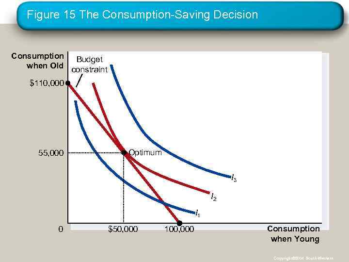 Figure 15 The Consumption-Saving Decision Consumption Budget when Old constraint $110, 000 55, 000 Optimum I 3 I 2 I 1 0 $50, 000 100, 000 Consumption when Young Copyright© 2004 South-Western
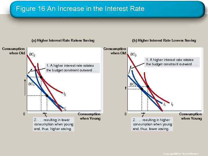 Figure 16 An Increase in the Interest Rate (a) Higher Interest Rate Raises Saving Consumption when Old (b) Higher Interest Rate Lowers Saving Consumption when Old BC 2 1. A higher interest rate rotates the budget constraint outward. . . BC 1 I 2 I 1 0 2. . resulting in lower consumption when young and, thus, higher saving. Consumption when Young 0 2. . resulting in higher consumption when young and, thus, lower saving. Consumption when Young Copyright© 2004 South-Western
 THREE APPLICATIONS • Thus, an increase in the interest rate could either encourage or discourage saving. Copyright© 2004 South-Western
 Summary • A consumer’s budget constraint shows the possible combinations of different goods he can buy given his income and the prices of the goods. • The slope of the budget constraint equals the relative price of the goods. • The consumer’s indifference curves represent his preferences. Copyright© 2004 South-Western
 Summary • Points on higher indifference curves are preferred to points on lower indifference curves. • The slope of an indifference curve at any point is the consumer’s marginal rate of substitution. • The consumer optimizes by choosing the point on his budget constraint that lies on the highest indifference curve. Copyright© 2004 South-Western
 Summary • When the price of a good falls, the impact on the consumer’s choices can be broken down into an income effect and a substitution effect. • The income effect is the change in consumption that arises because a lower price makes the consumer better off. • The income effect is reflected by the movement from a lower to a higher indifference curve. Copyright© 2004 South-Western
 Summary • The substitution effect is the change in consumption that arises because a price change encourages greater consumption of the good that has become relatively cheaper. • The substitution effect is reflected by a movement along an indifference curve to a point with a different slope. Copyright© 2004 South-Western
 Summary • The theory of consumer choice can explain: • Why demand curves can potentially slope upward. • How wages affect labor supply. • How interest rates affect household saving. Copyright© 2004 South-Western


