5 TRANSACTION COSTS AND MIP 5 1 Transaction

5. TRANSACTION COSTS AND MIP 5. 1 Transaction costs constraints in MVO 5. 2 Transaction costs penalty in quadratic utility 5. 3 Discrete constraints via mixed integer programming Reading: Scherer and Martin (2005), Chap. 3. 3* Chincirini and Kim (2006), Chap. 10. 1 – 10. 5, 10 A * This is included in a copy of Chap. 3. 2 & 3. 3 posted to the class web site. You should ignore 3. 2 except for optional casual reading at this point, and ignore all of the code in both sections as it was based on Rnuopt and this code will be replaced soon. 7/2/2013 Copyright R. Douglas Martin 1

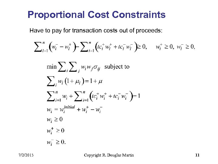
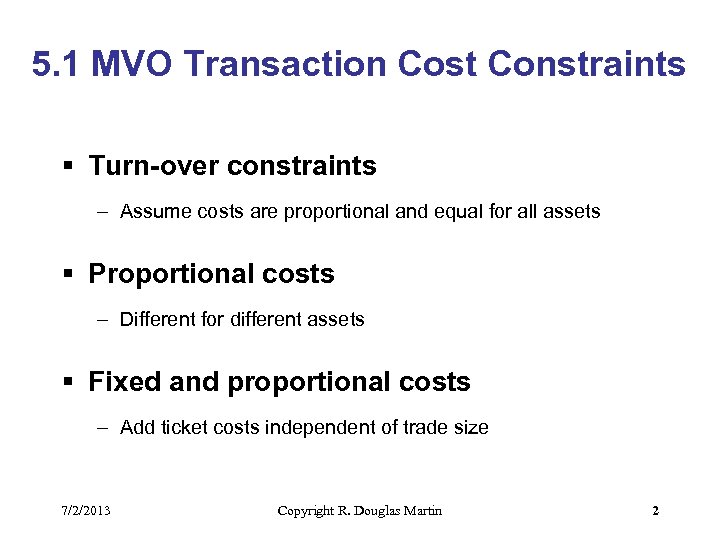5. 1 MVO Transaction Cost Constraints § Turn-over constraints – Assume costs are proportional and equal for all assets § Proportional costs – Different for different assets § Fixed and proportional costs – Add ticket costs independent of trade size 7/2/2013 Copyright R. Douglas Martin 2

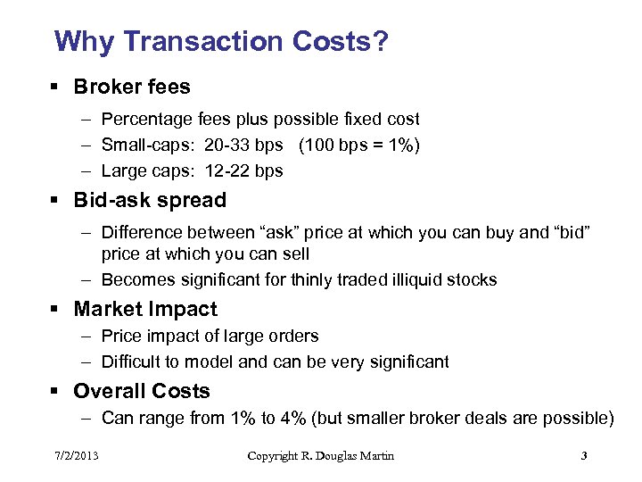Why Transaction Costs? § Broker fees – Percentage fees plus possible fixed cost – Small-caps: 20 -33 bps (100 bps = 1%) – Large caps: 12 -22 bps § Bid-ask spread – Difference between “ask” price at which you can buy and “bid” price at which you can sell – Becomes significant for thinly traded illiquid stocks § Market Impact – Price impact of large orders – Difficult to model and can be very significant § Overall Costs – Can range from 1% to 4% (but smaller broker deals are possible) 7/2/2013 Copyright R. Douglas Martin 3

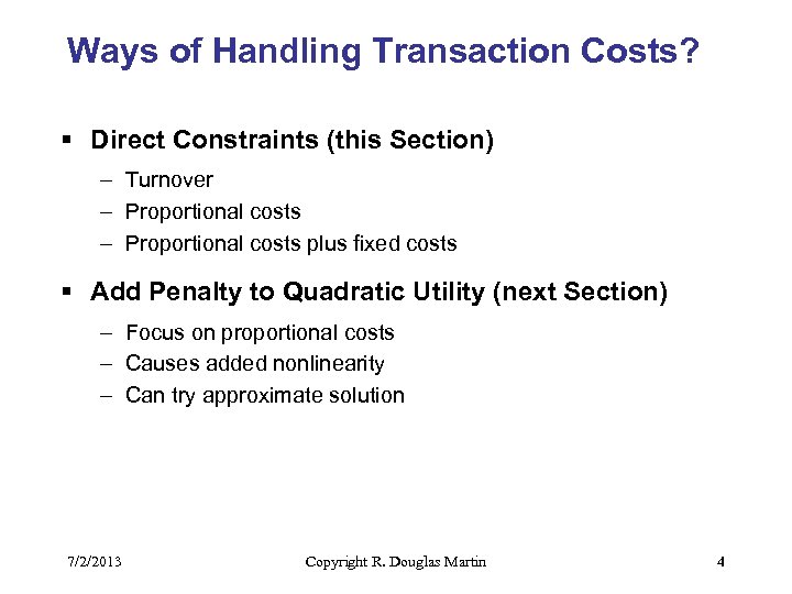Ways of Handling Transaction Costs? § Direct Constraints (this Section) – Turnover – Proportional costs plus fixed costs § Add Penalty to Quadratic Utility (next Section) – Focus on proportional costs – Causes added nonlinearity – Can try approximate solution 7/2/2013 Copyright R. Douglas Martin 4

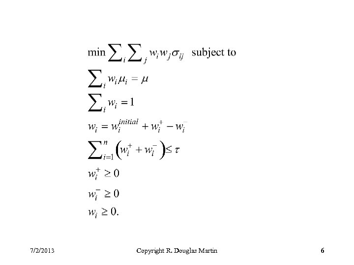
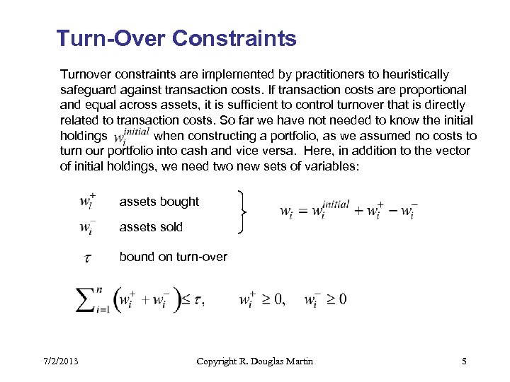Turn-Over Constraints Turnover constraints are implemented by practitioners to heuristically safeguard against transaction costs. If transaction costs are proportional and equal across assets, it is sufficient to control turnover that is directly related to transaction costs. So far we have not needed to know the initial holdings when constructing a portfolio, as we assumed no costs to turn our portfolio into cash and vice versa. Here, in addition to the vector of initial holdings, we need two new sets of variables: assets bought assets sold bound on turn-over 7/2/2013 Copyright R. Douglas Martin 5

7/2/2013 Copyright R. Douglas Martin 6

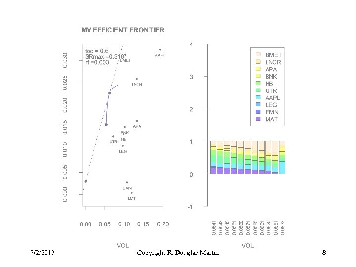
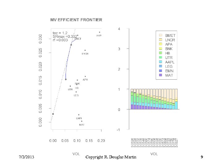
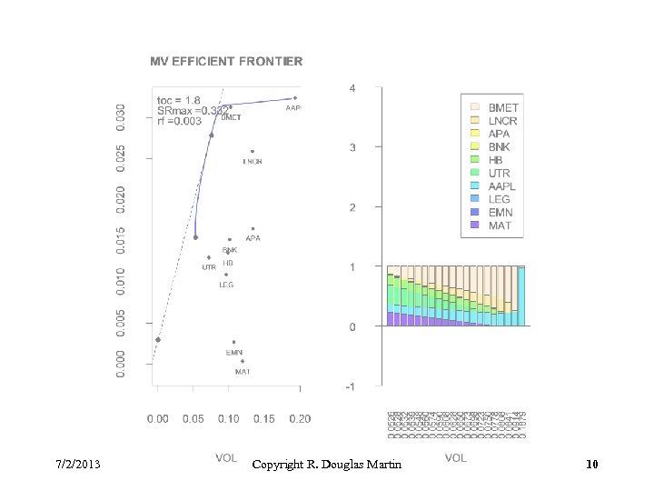
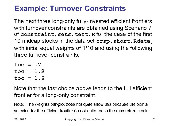Example: Turnover Constraints The next three long-only fully-invested efficient frontiers with turnover constraints are obtained using Scenario 7 of constraint. sets. test. R for the case of the first 10 midcap stocks in the data set crsp. short. Rdata, with initial equal weights of 1/10 and using the following three turnover constraints: toc =. 7 toc = 1. 2 toc = 1. 8 Note that the last choice above leads to the full efficient frontier for a long-only constraint. Note: The weights bar-plot does not quite show this because the points selected for the efficient frontier do not quite reach the max return stock. 7/2/2013 Copyright R. Douglas Martin 7

7/2/2013 Copyright R. Douglas Martin 8

7/2/2013 Copyright R. Douglas Martin 9

7/2/2013 Copyright R. Douglas Martin 10

Proportional Cost Constraints Have to pay for transaction costs out of proceeds: 7/2/2013 Copyright R. Douglas Martin 11

Example: Proportional Costs Constraints 7/2/2013 Copyright R. Douglas Martin 12

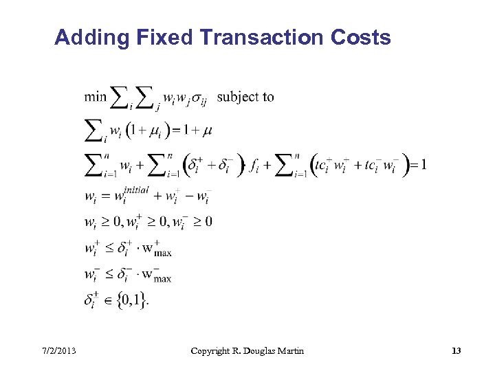Adding Fixed Transaction Costs 7/2/2013 Copyright R. Douglas Martin 13

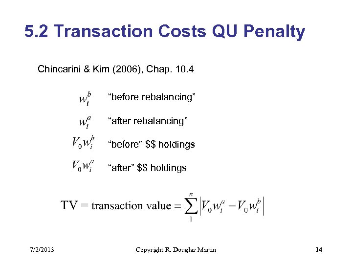5. 2 Transaction Costs QU Penalty Chincarini & Kim (2006), Chap. 10. 4 “before rebalancing” “after rebalancing” “before” $$ holdings “after” $$ holdings 7/2/2013 Copyright R. Douglas Martin 14

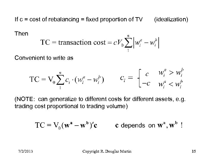If c = cost of rebalancing = fixed proportion of TV (idealization) Then Convenient to write as (NOTE: can generalize to different costs for different assets, e. g. trading cost proportional to trading volume) 7/2/2013 Copyright R. Douglas Martin 15

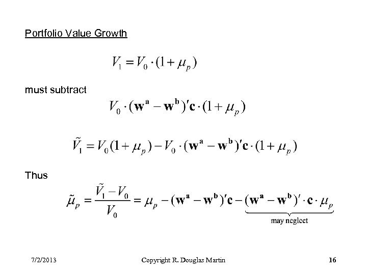Portfolio Value Growth must subtract Thus 7/2/2013 Copyright R. Douglas Martin 16

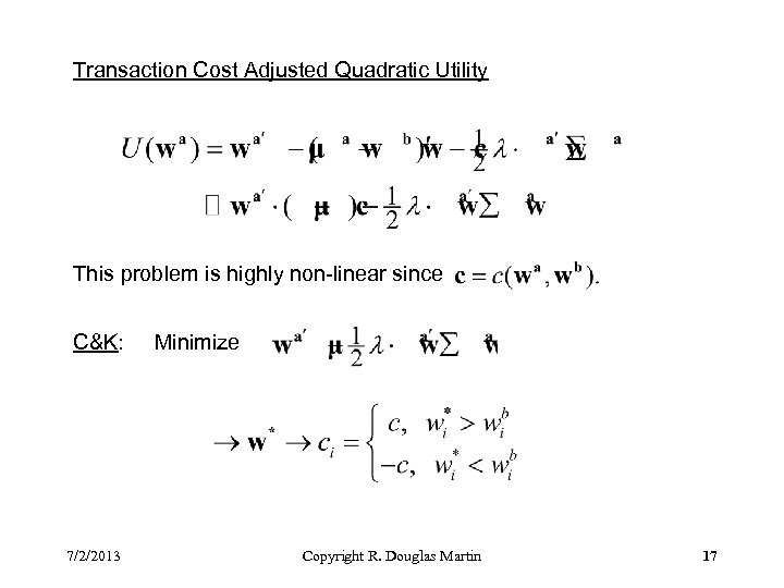Transaction Cost Adjusted Quadratic Utility This problem is highly non-linear since C&K: 7/2/2013 Minimize Copyright R. Douglas Martin 17

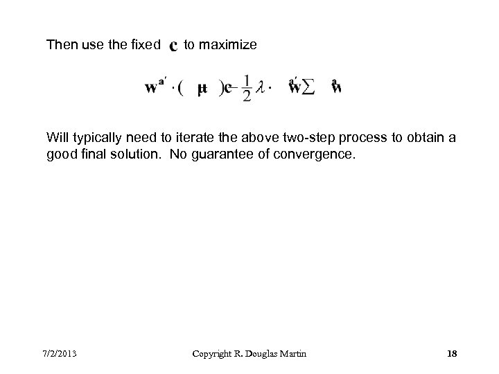Then use the fixed to maximize Will typically need to iterate the above two-step process to obtain a good final solution. No guarantee of convergence. 7/2/2013 Copyright R. Douglas Martin 18

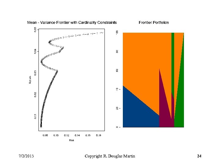
5. 3 Discrete Constraints via MIP § Buy-in thresholds and cardinality constraints – Portfolio managers and their clients hate small positions – You only want 25 out of 500 stocks with bounds on weights § Requires mixed integer programming (MIP) § Mathematical problem formulation § Example with pure cardinality constraint – Best 2 out of 4 stocks – Non-convex efficient frontier 7/2/2013 Copyright R. Douglas Martin 19

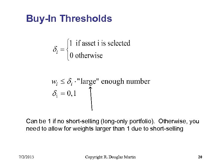Buy-In Thresholds Can be 1 if no short-selling (long-only portfolio). Otherwise, you need to allow for weights larger than 1 due to short-selling 7/2/2013 Copyright R. Douglas Martin 20

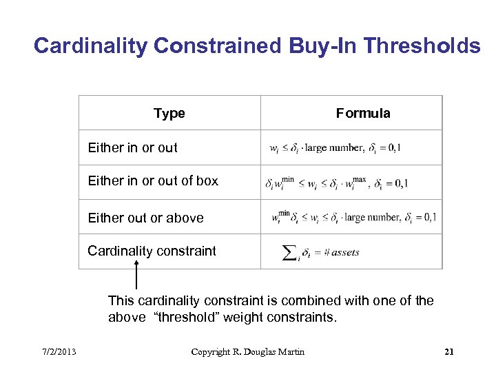Cardinality Constrained Buy-In Thresholds Type Formula Either in or out of box Either out or above Cardinality constraint This cardinality constraint is combined with one of the above “threshold” weight constraints. 7/2/2013 Copyright R. Douglas Martin 21

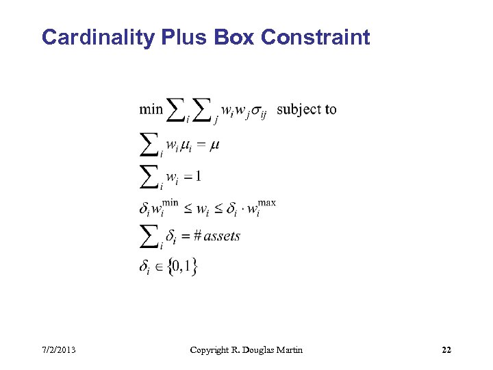Cardinality Plus Box Constraint 7/2/2013 Copyright R. Douglas Martin 22

Best 2 Out of 4 Long-Only Example 4 uncorrelated assets with multivariate normal distribution having common variances of 20% and mean returns of 2%, 4%, 5%, 8%. T = 50 sets of simulated returns Example on next slide was produced with Rnuopt and will be replaced with example based on alternative R optimizer. 7/2/2013 Copyright R. Douglas Martin 23

7/2/2013 Copyright R. Douglas Martin 24