5 -Minute Check on section 7 -2 b

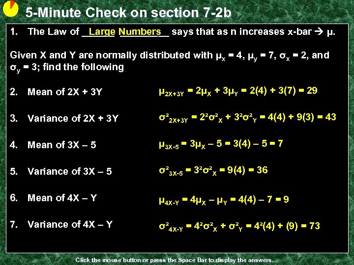
5 -Minute Check on section 7 -2 b Large Numbers 1. The Law of _________ says that as n increases x-bar μ. Given X and Y are normally distributed with μx = 4, μy = 7, σx = 2, and σy = 3; find the following 2. Mean of 2 X + 3 Y μ 2 X+3 Y = 2μX + 3μY = 2(4) + 3(7) = 29 3. Variance of 2 X + 3 Y σ² 2 X+3 Y = 2²σ²X + 3²σ²Y = 4(4) + 9(3) = 43 4. Mean of 3 X – 5 μ 3 X-5 = 3μX – 5 = 3(4) – 5 = 7 5. Variance of 3 X – 5 σ² 3 X-5 = 3²σ²X = 9(4) = 36 6. Mean of 4 X – Y μ 4 X-Y = 4μX – μY = 4(4) – 7 = 9 7. Variance of 4 X – Y σ² 4 X-Y = 4²σ²X + σ²Y = 4²(4) + (9) = 73 Click the mouse button or press the Space Bar to display the answers.

Lesson 7 - R Review of Random Variables

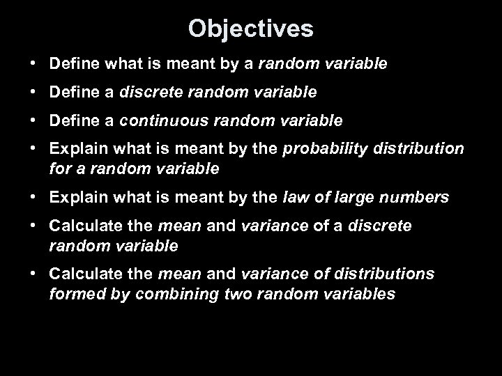
Objectives • Define what is meant by a random variable • Define a discrete random variable • Define a continuous random variable • Explain what is meant by the probability distribution for a random variable • Explain what is meant by the law of large numbers • Calculate the mean and variance of a discrete random variable • Calculate the mean and variance of distributions formed by combining two random variables

Vocabulary • Nothing

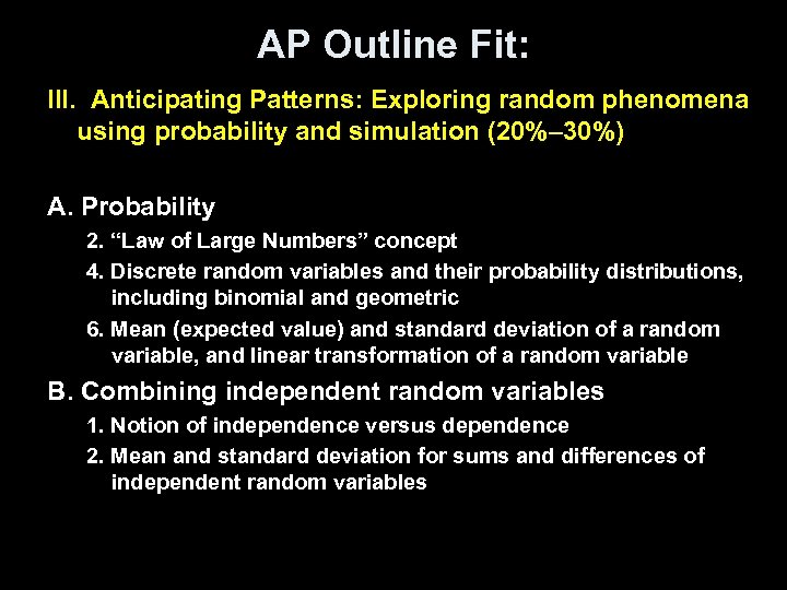
AP Outline Fit: III. Anticipating Patterns: Exploring random phenomena using probability and simulation (20%– 30%) A. Probability 2. “Law of Large Numbers” concept 4. Discrete random variables and their probability distributions, including binomial and geometric 6. Mean (expected value) and standard deviation of a random variable, and linear transformation of a random variable B. Combining independent random variables 1. Notion of independence versus dependence 2. Mean and standard deviation for sums and differences of independent random variables

What we Learned • Random Variables – Recognize and define a discrete random variable, and construct a probability distribution table and a probability histogram for the random variable – Recognize and define a continuous random variable, and determine probabilities of events as areas under density curves – Given a Normal random variable, use the standard Normal table or a graphing calculator to find probabilities of events as areas under the standard Normal distribution curve

What we Learned • Means and Variances of Random Variables – Calculate the mean and variance of a discrete random variable. Find the expected payout in a raffle or similar game of chance – Use simulation methods and the law of large numbers to approximate the mean of a distribution – Use rules for means and rules for variances to solve problems involving sums, differences, and linear combinations of random variables

Using your TI-83 calculator We can use 1 -Var-Stats to calculate the mean and standard deviation of a discrete random variable given it’s outcomes and probability • Type in outcomes in L 1 • Type in corresponding probabilities in L 2 • Use 1 -Var-Stats L 1, L 2 to get statistics • Notes: – Discrete Random Variables have countable (finite) values – Continuous Random Variables have an interval of values (infinite) – Ranges of Random Variables are determined by minimum or maximum values that they can take on

Discrete Random Variable - Mean The mean, or expected value [E(x)], of a discrete random variable is given by the formula μx = ∑ [x ∙P(x)] where x is the value of the random variable and P(x) is the probability of observing x (multiply them together and add all of them up) Mean of a Discrete Random Variable Interpretation: If we run an experiment over and over again, the law of large numbers helps us conclude that the difference between x and ux gets closer to 0 as n (number of repetitions) increases

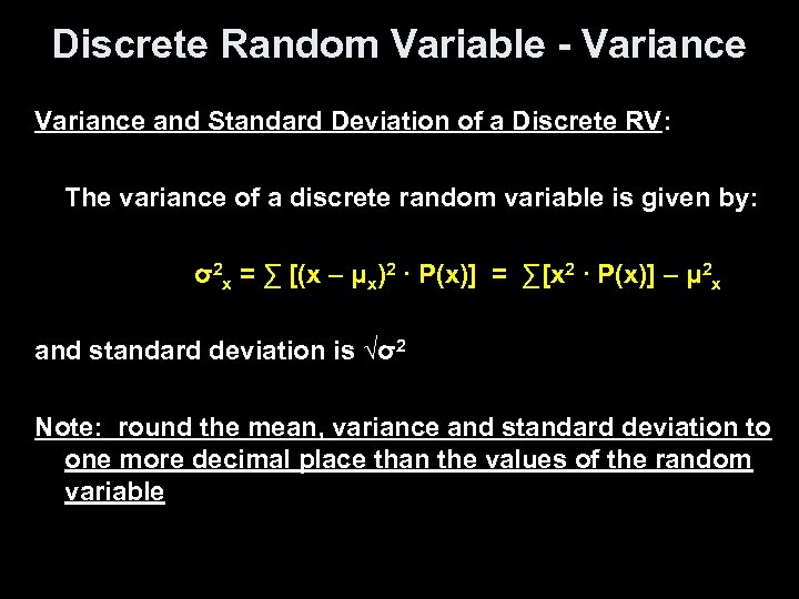
Discrete Random Variable - Variance and Standard Deviation of a Discrete RV: The variance of a discrete random variable is given by: σ2 x = ∑ [(x – μx)2 ∙ P(x)] = ∑[x 2 ∙ P(x)] – μ 2 x and standard deviation is √σ2 Note: round the mean, variance and standard deviation to one more decimal place than the values of the random variable

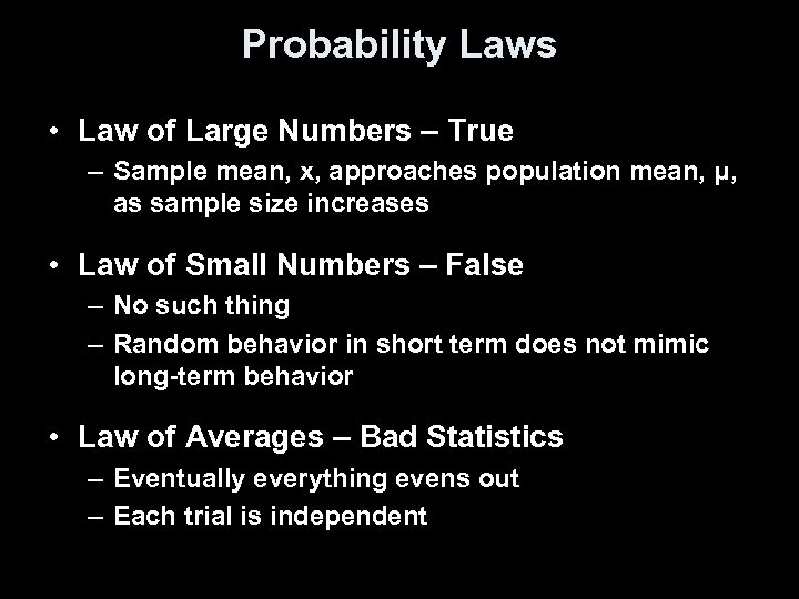
Probability Laws • Law of Large Numbers – True – Sample mean, x, approaches population mean, μ, as sample size increases • Law of Small Numbers – False – No such thing – Random behavior in short term does not mimic long-term behavior • Law of Averages – Bad Statistics – Eventually everything evens out – Each trial is independent

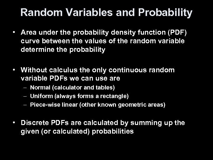
Random Variables and Probability • Area under the probability density function (PDF) curve between the values of the random variable determine the probability • Without calculus the only continuous random variable PDFs we can use are – Normal (calculator and tables) – Uniform (always forms a rectangle) – Piece-wise linear (other known geometric areas) • Discrete PDFs are calculated by summing up the given (or calculated) probabilities

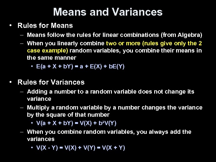
Means and Variances • Rules for Means – Means follow the rules for linear combinations (from Algebra) – When you linearly combine two or more (rules give only the 2 case example) random variables, you combine their means in the same manner • E(a + X + b. Y) = a + E(X) + b. E(Y) • Rules for Variances – Adding a number to a random variable does not change its variance – Multiply a random variable by a number changes the variance by the square of that number • V(a + X + b. Y) = V(X) + b²V(Y) – When you combine random variables, you always add the variances • V(X - Y) = V(X) + V(Y) = V(X + Y)

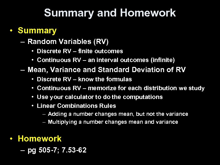
Summary and Homework • Summary – Random Variables (RV) • Discrete RV – finite outcomes • Continuous RV – an interval outcomes (infinite) – Mean, Variance and Standard Deviation of RV • • Discrete RV – know the formulas Continuous RV – memorize for each distribution we study Use your calculator to do the computations Linear Combinations Rules – Adding a number changes mean, but not the variance – Multiplying a number changes mean and variance • Homework – pg 505 -7; 7. 53 -62

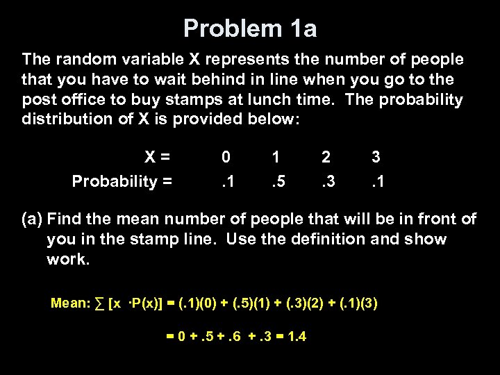
Problem 1 a The random variable X represents the number of people that you have to wait behind in line when you go to the post office to buy stamps at lunch time. The probability distribution of X is provided below: X = Probability = 0. 1 1. 5 2. 3 3. 1 (a) Find the mean number of people that will be in front of you in the stamp line. Use the definition and show work. Mean: ∑ [x ∙P(x)] = (. 1)(0) + (. 5)(1) + (. 3)(2) + (. 1)(3) = 0 +. 5 +. 6 +. 3 = 1. 4

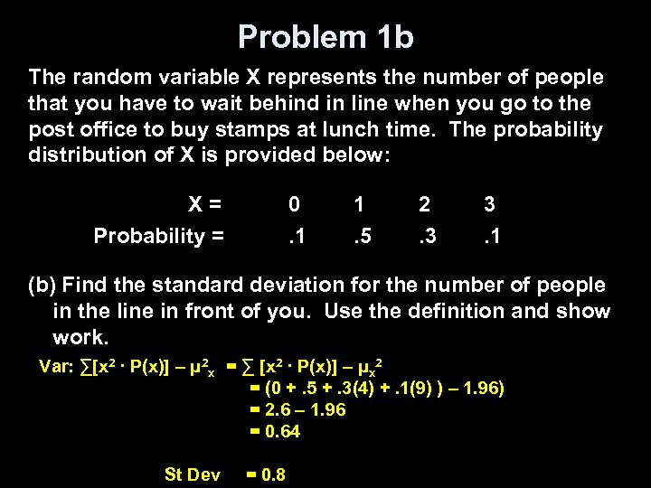
Problem 1 b The random variable X represents the number of people that you have to wait behind in line when you go to the post office to buy stamps at lunch time. The probability distribution of X is provided below: X = Probability = 0. 1 1. 5 2. 3 3. 1 (b) Find the standard deviation for the number of people in the line in front of you. Use the definition and show work. Var: ∑[x 2 ∙ P(x)] – μ 2 x = ∑ [x 2 ∙ P(x)] – μx 2 = (0 +. 5 +. 3(4) +. 1(9) ) – 1. 96) = 2. 6 – 1. 96 = 0. 64 St Dev = 0. 8

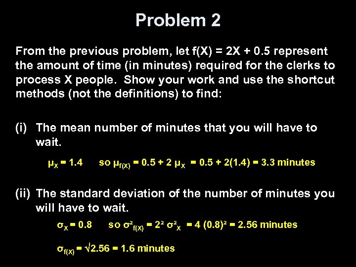
Problem 2 From the previous problem, let f(X) = 2 X + 0. 5 represent the amount of time (in minutes) required for the clerks to process X people. Show your work and use the shortcut methods (not the definitions) to find: (i) The mean number of minutes that you will have to wait. μX = 1. 4 so μf(X) = 0. 5 + 2 μX = 0. 5 + 2(1. 4) = 3. 3 minutes (ii) The standard deviation of the number of minutes you will have to wait. σX = 0. 8 so σ²f(X) = 2² σ²X = 4 (0. 8)² = 2. 56 minutes σf(X) = 2. 56 = 1. 6 minutes

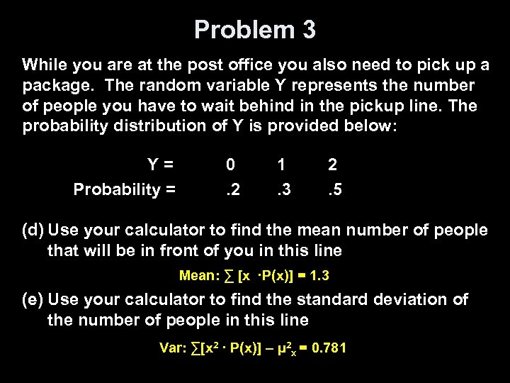
Problem 3 While you are at the post office you also need to pick up a package. The random variable Y represents the number of people you have to wait behind in the pickup line. The probability distribution of Y is provided below: Y = Probability = 0. 2 1. 3 2. 5 (d) Use your calculator to find the mean number of people that will be in front of you in this line Mean: ∑ [x ∙P(x)] = 1. 3 (e) Use your calculator to find the standard deviation of the number of people in this line Var: ∑[x 2 ∙ P(x)] – μ 2 x = 0. 781

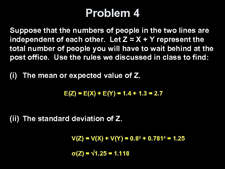
Problem 4 Suppose that the numbers of people in the two lines are independent of each other. Let Z = X + Y represent the total number of people you will have to wait behind at the post office. Use the rules we discussed in class to find: (i) The mean or expected value of Z. E(Z) = E(X) + E(Y) = 1. 4 + 1. 3 = 2. 7 (ii) The standard deviation of Z. V(Z) = V(X) + V(Y) = 0. 8² + 0. 781² = 1. 25 σ(Z) = 1. 25 = 1. 118

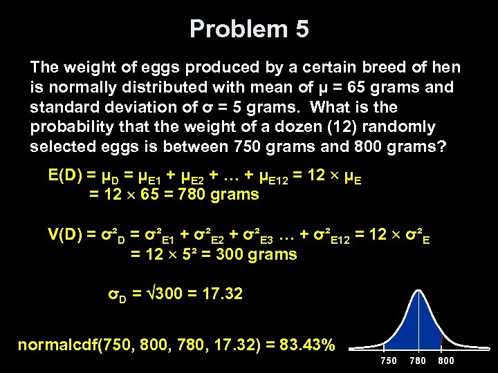
Problem 5 The weight of eggs produced by a certain breed of hen is normally distributed with mean of μ = 65 grams and standard deviation of σ = 5 grams. What is the probability that the weight of a dozen (12) randomly selected eggs is between 750 grams and 800 grams? E(D) = μD = μE 1 + μE 2 + … + μE 12 = 12 μE = 12 65 = 780 grams V(D) = σ²D = σ²E 1 + σ²E 2 + σ²E 3 … + σ²E 12 = 12 σ²E = 12 5² = 300 grams σD = 300 = 17. 32 normalcdf(750, 800, 780, 17. 32) = 83. 43% 750 780 800