5 1 Rates of Return 5 -1

5. 1 Rates of Return 5 -1

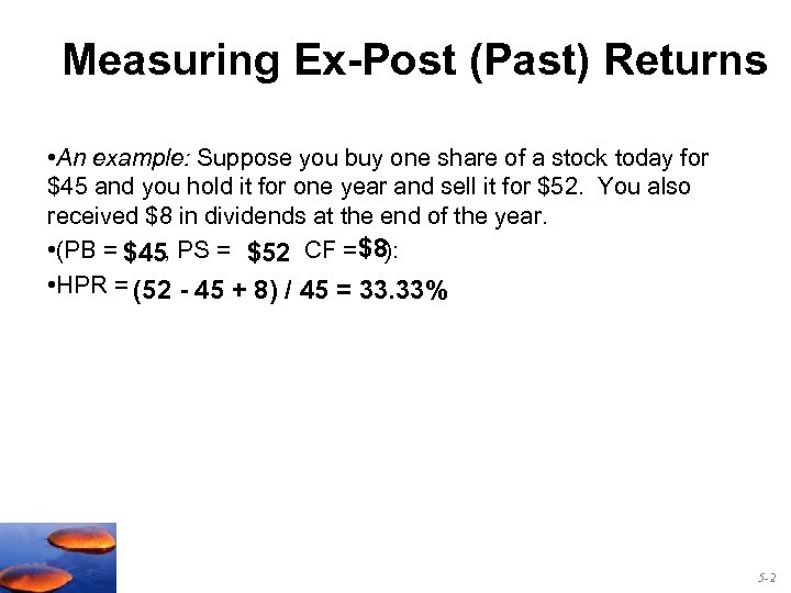Measuring Ex-Post (Past) Returns • An example: Suppose you buy one share of a stock today for $45 and you hold it for one year and sell it for $52. You also received $8 in dividends at the end of the year. • (PB = $45, PS = $52 CF = $8): , • HPR = (52 - 45 + 8) / 45 = 33. 33% 5 -2

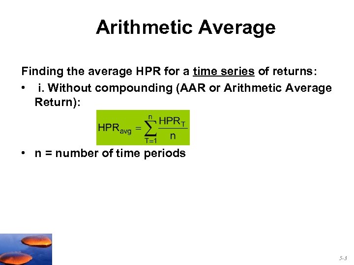Arithmetic Average Finding the average HPR for a time series of returns: • i. Without compounding (AAR or Arithmetic Average Return): • n = number of time periods 5 -3

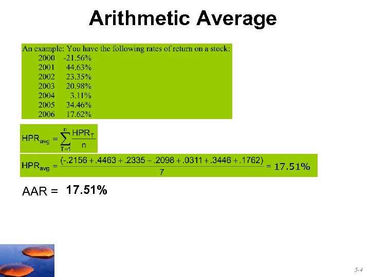Arithmetic Average 17. 51% AAR = 17. 51% 5 -4

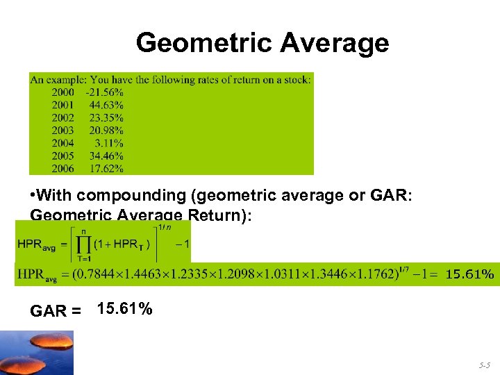Geometric Average • With compounding (geometric average or GAR: Geometric Average Return): 15. 61% GAR = 15. 61% 5 -5

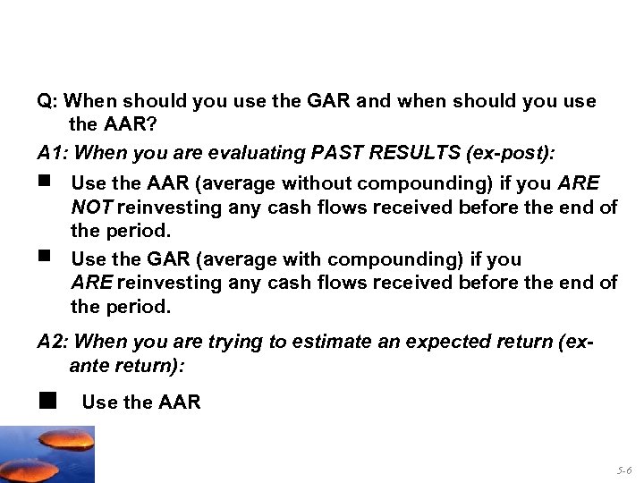Q: When should you use the GAR and when should you use the AAR? A 1: When you are evaluating PAST RESULTS (ex-post): n Use the AAR (average without compounding) if you ARE NOT reinvesting any cash flows received before the end of the period. n Use the GAR (average with compounding) if you ARE reinvesting any cash flows received before the end of the period. A 2: When you are trying to estimate an expected return (exante return): n Use the AAR 5 -6

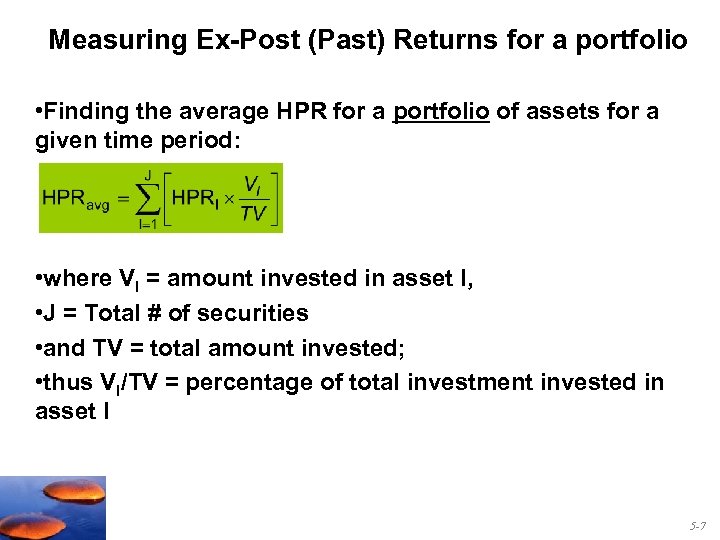Measuring Ex-Post (Past) Returns for a portfolio • Finding the average HPR for a portfolio of assets for a given time period: • where VI = amount invested in asset I, • J = Total # of securities • and TV = total amount invested; • thus VI/TV = percentage of total investment invested in asset I 5 -7

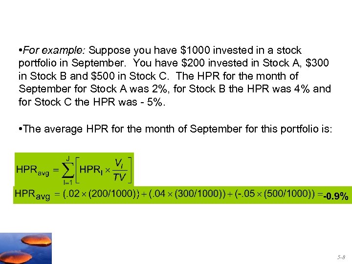• For example: Suppose you have $1000 invested in a stock portfolio in September. You have $200 invested in Stock A, $300 in Stock B and $500 in Stock C. The HPR for the month of September for Stock A was 2%, for Stock B the HPR was 4% and for Stock C the HPR was - 5%. • The average HPR for the month of September for this portfolio is: -0. 9% 5 -8

5. 2 Risk and Risk Premiums 5 -9

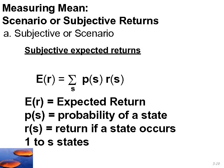Measuring Mean: Scenario or Subjective Returns a. Subjective or Scenario Subjective expected returns E(r) = S p(s) r(s) s E(r) = Expected Return p(s) = probability of a state r(s) = return if a state occurs 1 to s states 5 -10

Measuring Variance or Dispersion of Returns a. Subjective or Scenario Variance = [ 2]1/2 E(r) = Expected Return p(s) = probability of a state rs = return in state “s” 5 -11

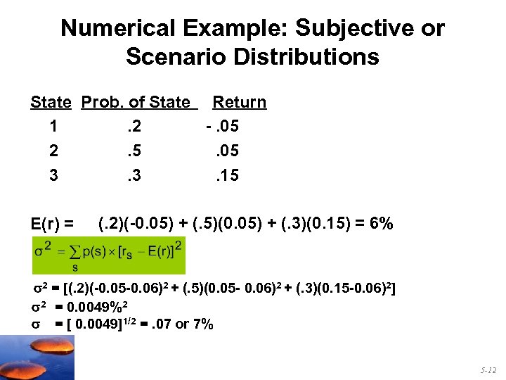Numerical Example: Subjective or Scenario Distributions State Prob. of State Return 1. 2 -. 05 2. 5. 05 3. 3. 15 E(r) = (. 2)(-0. 05) + (. 5)(0. 05) + (. 3)(0. 15) = 6% 2 = [(. 2)(-0. 05 -0. 06)2 + (. 5)(0. 05 - 0. 06)2 + (. 3)(0. 15 -0. 06)2] 2 = 0. 0049%2 = [ 0. 0049]1/2 =. 07 or 7% 5 -12

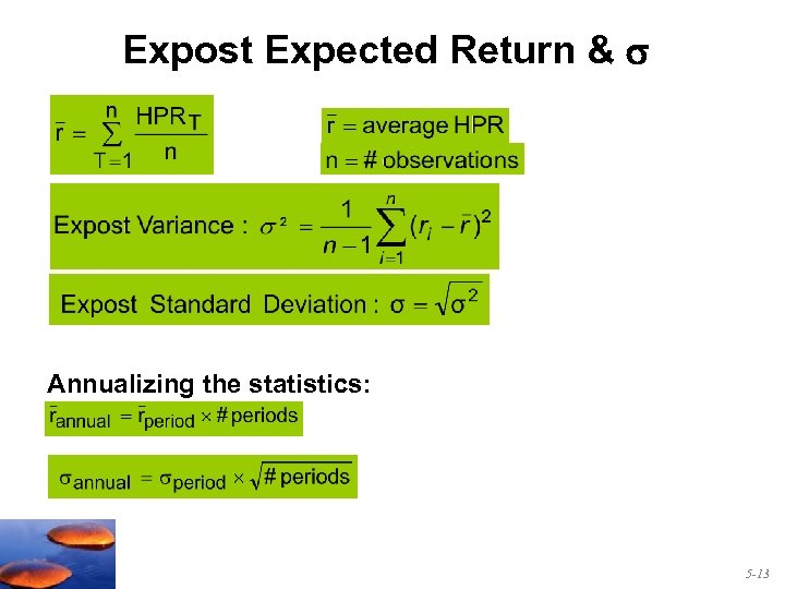Expost Expected Return & Annualizing the statistics: 5 -13

Using Ex-Post Returns to estimate Expected HPR Estimating Expected HPR (E[r]) from ex-post data. Use the arithmetic average of past returns as a forecast of expected future returns and, Perhaps apply some (usually ad-hoc) adjustment to past returns Problems? • Which historical time period? • Have to adjust for current economic situation 5 -14

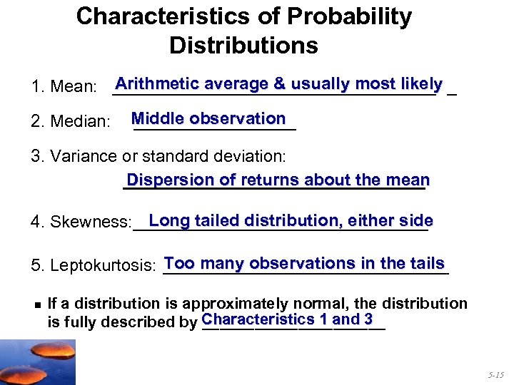Characteristics of Probability Distributions Arithmetic average & usually most likely 1. Mean: _________________ _ 2. Median: Middle observation _________ 3. Variance or standard deviation: Dispersion of returns about the mean Long tailed distribution, either side 4. Skewness: ________________ Too many observations in the tails 5. Leptokurtosis: _______________ n If a distribution is approximately normal, the distribution is fully described by Characteristics 1 and 3 ___________ 5 -15

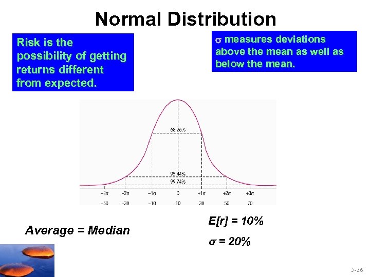Normal Distribution Risk is the possibility of getting returns different from expected. Average = Median measures deviations above the mean as well as below the mean. E[r] = 10% = 20% 5 -16

5. 3 The Historical Record 5 -17

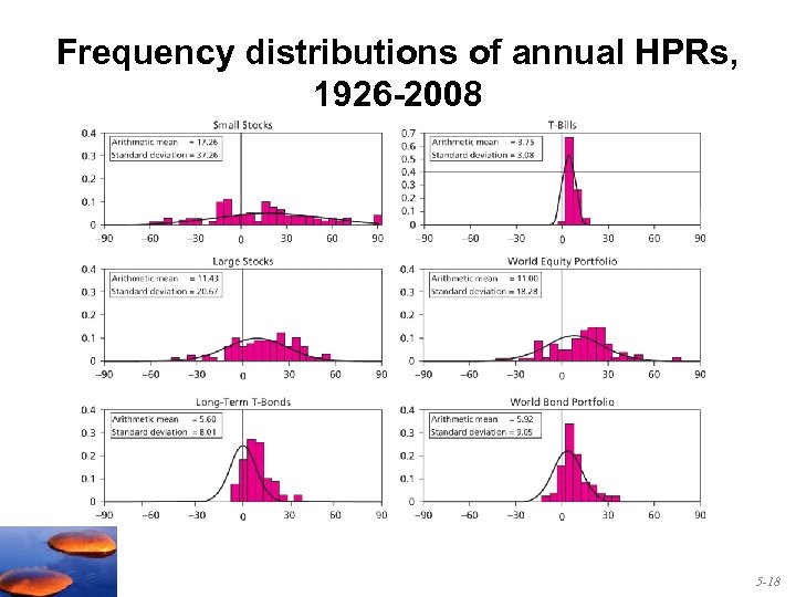Frequency distributions of annual HPRs, 1926 -2008 5 -18

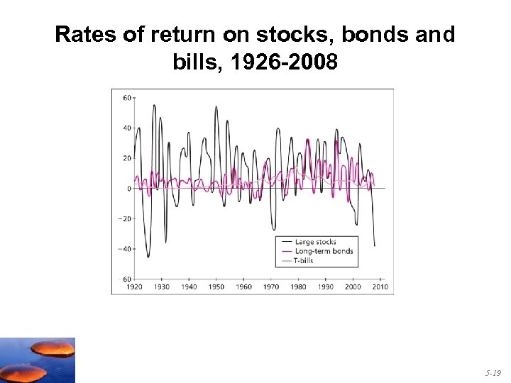Rates of return on stocks, bonds and bills, 1926 -2008 5 -19

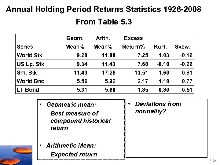Annual Holding Period Returns Statistics 1926 -2008 From Table 5. 3 Geom. Excess Mean% Series Arith. Mean% Return% Kurt. Skew. World Stk 9. 20 11. 00 7. 25 1. 03 -0. 16 US Lg. Stk 9. 34 11. 43 7. 68 -0. 10 -0. 26 11. 43 17. 26 13. 51 1. 60 0. 81 World Bnd 5. 56 5. 92 2. 17 1. 10 0. 77 LT Bond 5. 31 5. 60 1. 85 0. 80 0. 51 Sm. Stk • Geometric mean: Best measure of compound historical return • Deviations from normality? • Arithmetic Mean: Expected return 5 -20

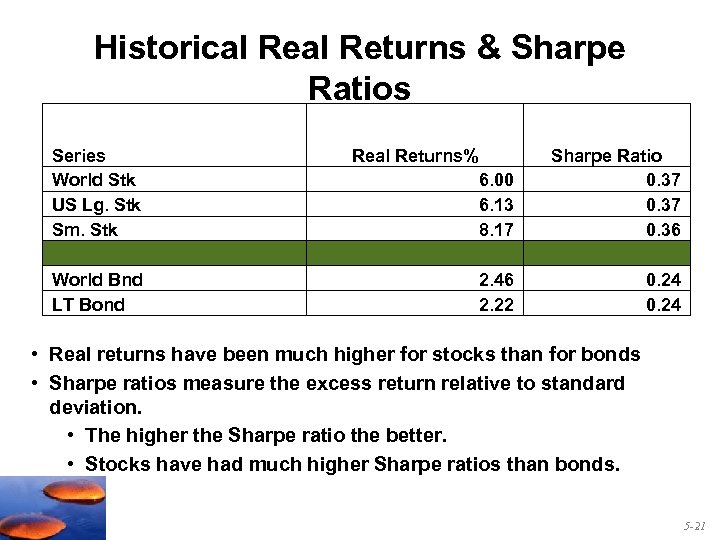Historical Returns & Sharpe Ratios Series World Stk US Lg. Stk Sm. Stk World Bnd LT Bond Real Returns% 6. 00 6. 13 8. 17 Sharpe Ratio 0. 37 0. 36 2. 46 2. 22 0. 24 • Real returns have been much higher for stocks than for bonds • Sharpe ratios measure the excess return relative to standard deviation. • The higher the Sharpe ratio the better. • Stocks have had much higher Sharpe ratios than bonds. 5 -21

5. 4 Inflation and Real Rates of Return 5 -22

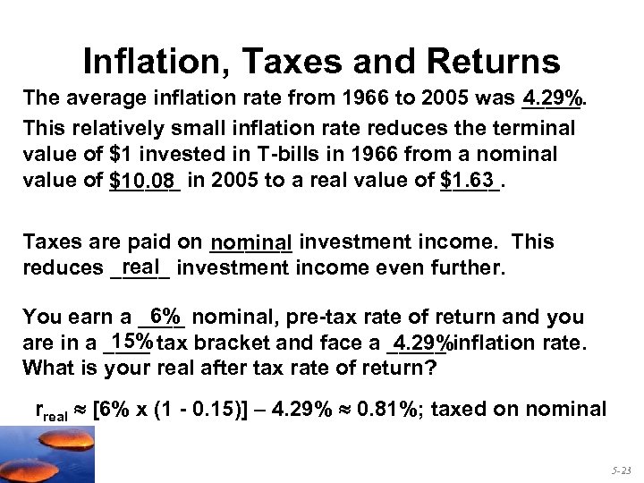Inflation, Taxes and Returns The average inflation rate from 1966 to 2005 was _____. 4. 29% This relatively small inflation rate reduces the terminal value of $1 invested in T-bills in 1966 from a nominal value of ______ in 2005 to a real value of $1. 63 _____. $10. 08 Taxes are paid on _______ investment income. This nominal reduces _____ investment income even further. 6% You earn a ____ nominal, pre-tax rate of return and you 15% are in a ____ tax bracket and face a _____ inflation rate. 4. 29% What is your real after tax rate of return? rreal [6% x (1 - 0. 15)] – 4. 29% 0. 81%; taxed on nominal 5 -23

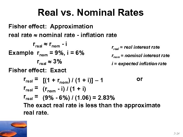Real vs. Nominal Rates Fisher effect: Approximation real rate nominal rate - inflation rate rreal rnom - i rreal = real interest rate Example rnom = 9%, i = 6% rnom = nominal interest rate rreal 3% i = expected inflation rate Fisher effect: Exact rreal = [(1 + rnom) / (1 + i)] – 1 or rreal = (rnom - i) / (1 + i) rreal = (9% - 6%) / (1. 06) = 2. 83% The exact real rate is less than the approximate real rate. 5 -24