452 NWP 2017 Major Steps in the

452 NWP 2017

Major Steps in the Forecast Process • • Data Collection Quality Control Data Assimilation Model Integration Post Processing of Model Forecasts Human Interpretation (sometimes) Product and graphics generation

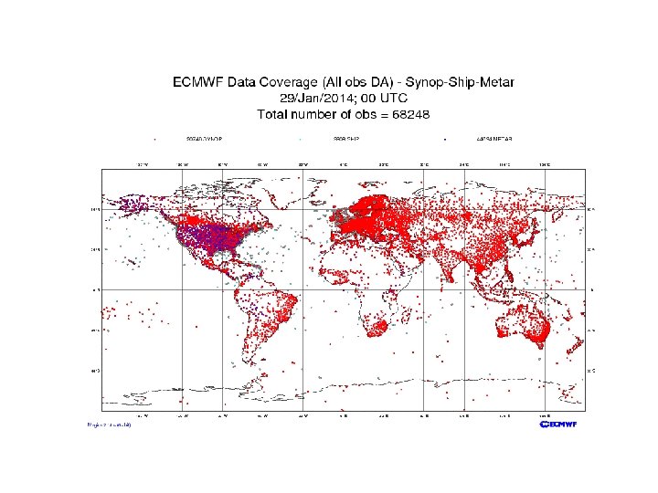
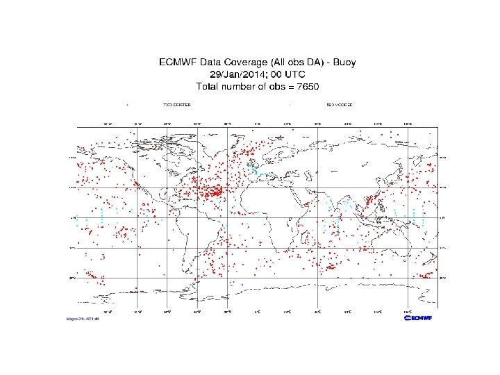
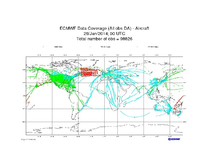
Data Collection • Weather is observed throughout the world and the data is distributed in real time. • Many types of data and networks, including: – – – – Surface observations from many sources Radiosondes and radar profilers Fixed and drifting buoys Ship observations Aircraft observations Satellite soundings Cloud and water vapor track winds Radar and satellite imagery

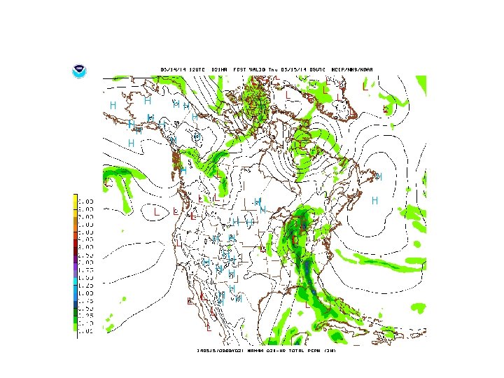
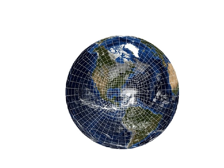
Observation and Data Collection

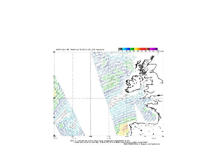
Atmospheric Moisture Vectors

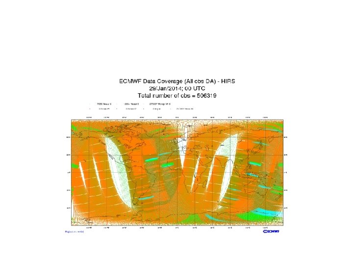
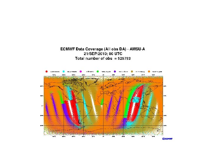
Weather Satellites Are Now 99% of the Data Assets Used for NWP • Geostationary Satellites: Imagery, soundings, cloud and water vapor winds • Polar Orbiter Satellites: Imagery, soundings, many wavelengths • RO (GPS) satellites • Scatterometers • Active radars in space (GPM)

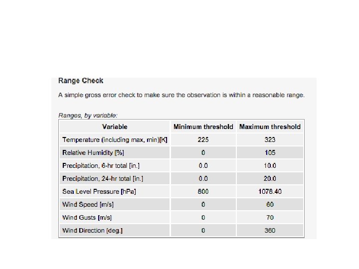
Quality Control • Automated algorithms and manual intervention to detect, correct, and remove errors in observed data. • Examples: – Range check – Buddy check – Comparison to first guess fields from previous model run – Hydrostatic and vertical consistency checks for soundings. • A very important issue for a forecaster--sometimes good data is rejected and vice versa.

3 March 1999: Forecast a snowstorm … got a windstorm instead Eta 48 hr SLP Forecast valid 00 UTC 3 March 1999

Pacific Analysis At 4 PM 18 November 2003 Bad Observation

Forecaster Involvement • A good forecast is on the lookout for NWP systems rejecting bad data, particularly in data sparse areas. • Quality control systems can allow models to go off to never land. • Less of a problem today due to satellite data everywhere.

Objective Analysis/Data Assimilation • Observations are scattered in three dimensions • Numerical weather models are generally solved on a three-dimensional grid • Need to interpolate observations to grid points and to ensure that the various fields are consistent and physically plausible (e. g. , most of the atmosphere in hydrostatic and gradient wind balance).

Objective Analysis • Interpolation of observational data to either a grid (most often!) or some basis function (e. g. , spectral components) • Typically iterative (done in several passes)

Objective Analysis/Data Assimilation • Often starts with a “first guess”, usually the gridded forecast from an earlier run (frequently a run starting 6 hr earlier) • This first guess is then modified by the observations. • Adjustments are made to insure proper balance. • Often iterative

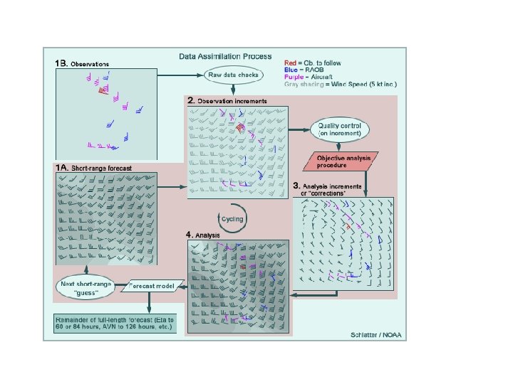
An early objective analysis scheme is the Cressman scheme

3 DVAR: 3 D Variational Data Assimilation • Used by the National Weather Service today for the GFS and NAM (called GSI) • Tries to create an analysis that minimizes a cost function dependent on the difference between the analysis and (1) first guess and (2) observations • Does this at a single time.

3 DVAR Covariances: Spreads Error in Space

4 DVAR: Four Dimension Variational Data Assimilation • Tries to optimize analyses at MULTIPLE TIMES • Tries to duplicate the observed evolution over time as well as the situation at initialization time. • Uses the model itself as a data assimilation too.

4 DVAR Components • Full non-linear model • Tangent linear version of the full model (linearized version of the forecast model) • Adjoint of the tangent linear model -which allows one to integrate the model backwards. Tells sensitivity of final state to the initial state.

4 DVAR • Typical runs the model back and forth during an initialization period (6 -12 hr), roughly ten times. • Substantial computational cost. • Need to have adjoint and TL version of the model. • Currently used by ECMWF, CMC, UKMET, and US Navy. NOT NCEP.

Many of the next generation data assimilation approaches are ensemble based • Example: the Ensemble Kalman Filter (En. KF)

Mesoscale Covariances 12 Z January 24, 2004 Camano Island Radar |V 950|-qr covariance

Surface Pressure Covariance Land Ocean

An Attractive Option: En. KF Temperature observation 3 DVAR En. KF

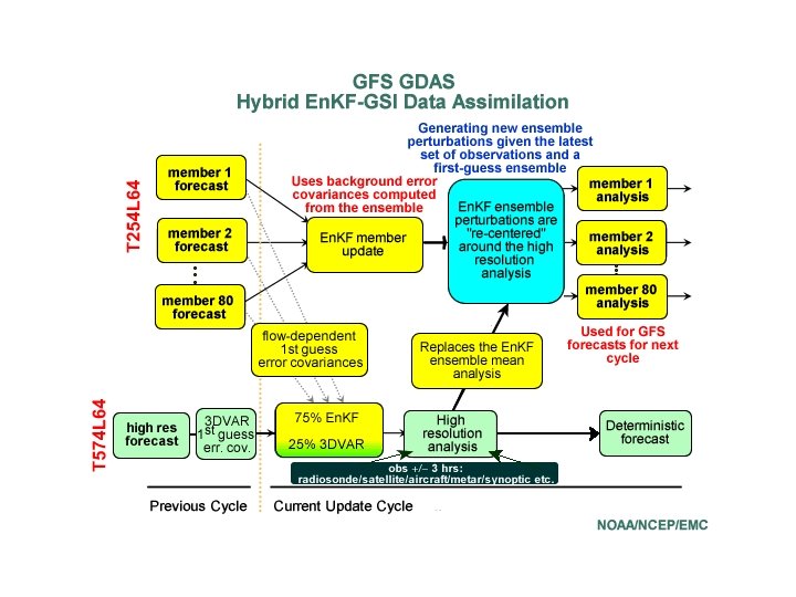
Hybrid Data Assimilation: Now Used in GFS • Uses both 3 DVAR and Enk. F • Uses Enk. F covariances from GFS ensemble in 3 DVAR.

Next Advance ENVAR • Use temporal covariances to spread impact of observations over TIME. • Now operational. • Has some of the properties of 4 DVAR (adjusts model evolution)

Vertical Coordinates and Nesting

Vertical Coordinate Systems • Originally p and z: but they had a problem…BC when the grid hit terrain! • Then eta, sigma p and sigma z, theta • Increasingly use of hybrids– e. g. , sigmatheta

Sigma

Sigma-Theta

Nesting

Why Nesting? • Could run a model over the whole globe, but that would require large amounts of computational resource, particularly if done at high resolution. • Alternative is to only use high resolution where you need it…nesting is one approach. • In nesting, a small higher resolution domain is embedded with a larger, lower-resolution domain.

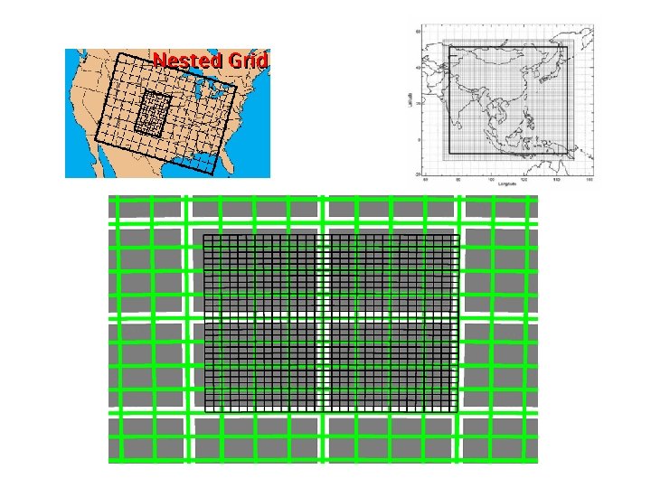
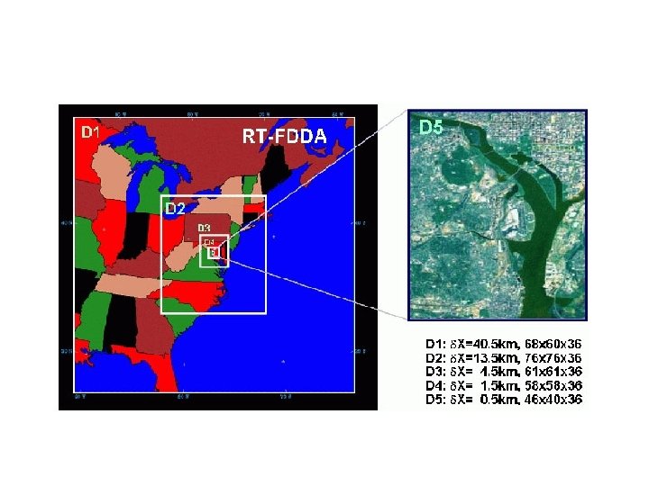
Nesting • Can be one-way or two way. • In the future, there will be adaptive nests that will put more resolution where it is needed. • And instead of rectangular grids, other shapes can be used.

Next Generation Global Models Under Development! • Will use different geometries

MPAS: Hexagonal Shapes

MPAS

FV 3 -Replacement for GFS

Major U. S. Models Overview • Global Models – Global Forecast System Model (GFS). Uses spectral representation rather than grids in the horizontal. Global, resolution equivalent to 13 km grid model. Run out to 384 hr, four times per day. – Navy Global Environmental Model (NAVGEM). 180 hour, four times a day. 50 levels, 37 km grid – UKMET Unified Model just taken on by U. S. Air Force. They call it the Global Air-Land Weather Exploitation Model (GALWEM)

Mesoscale Models • Mesoscale Models NMMB is the main NWS mesoscale model. They also use WRF-ARW (Advanced Research WRF, Weather Research Forecasting system). WRF-ARW is the main mesoscale modeling system that is used by the NWS and the university/research community. NMMB is run at 12 -km grid spacing, four times a day to 84 h. Also smaller 4 -km nests, single 1. 3 km nest. • COAMPS (Navy). The Navy mesoscale model. . similar to WRF but coupled to ocean model.

Major International NWP Centers • ECMWF: European Center for Medium. Range Weather Forecasting. The Gold standard. Their global model is considered the best. 9 km resolution • UK Met Office Unified Model: An excellent global model slightly superior to GFS • Canadian Meteorological Center • Other lesser centers

Global Forecast System (GFS) Model • Previous called the Aviation (AVN) and Medium Range Forecast (MRF) models. • Spectral global model and 64 levels • Relatively primitive microphysics. • Sophisticated surface physics and radiation • Run four times a day to 384 hr (16 days!). • Major increase in skill during past decades derived from using direct satellite radiance in the 3 DVAR analysis scheme and other satellite assets. • 13 km grid spacing equivalent over the first 10 days of the model forecast and 35 km from 10 to 16 days (384 hours). Thus, it now essentially a global mesoscale model

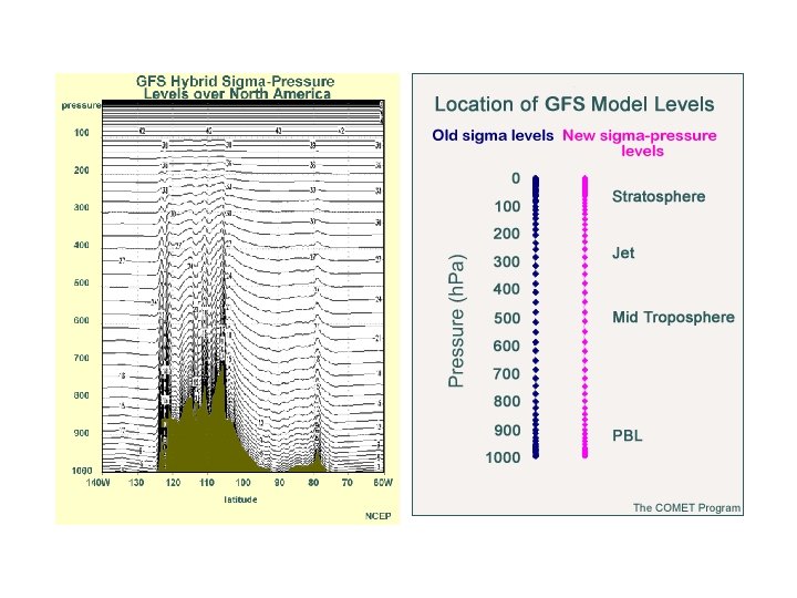
GFS • Vertical coordinates are hybrid sigma/pressure… sigma at low levels to pressure aloft.

GFS Data Assimilation (GDAS) • Global analysis every 6 hr • Has a later data cut-off time than the mesoscale models…and thus can get a higher percentage of data. • Uses much more satellite assets. . thus improve global analysis and forecasts. • Major gains in southern hemisphere • Hybrid Data assimilation based on 3 DVAR (called GSI) and GFE ensemble (next slide)

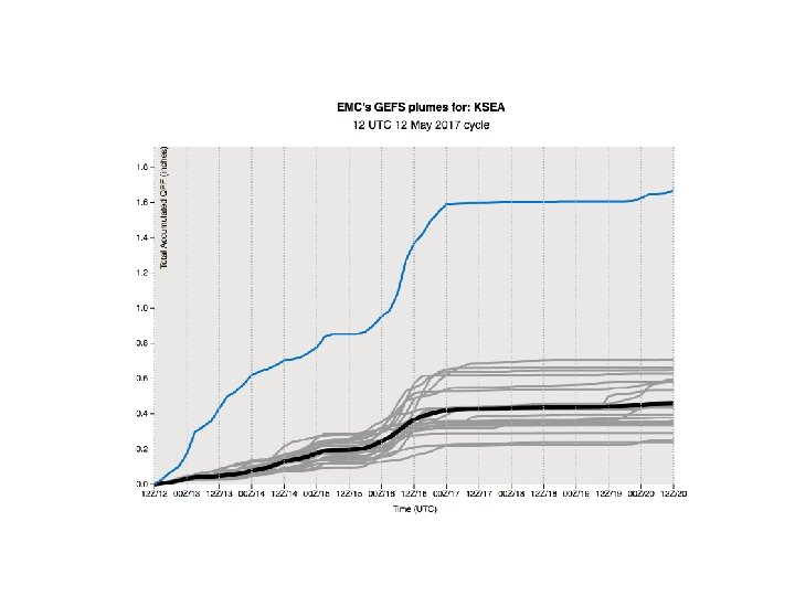
In addition to the high resolution GFS, there is a lower resolution GFS ensemble called GFE • • 34 km grid space equivalent 20 members Stochastic physics to help produce diversity 16 days

GFS Hybrid Data Assimilation

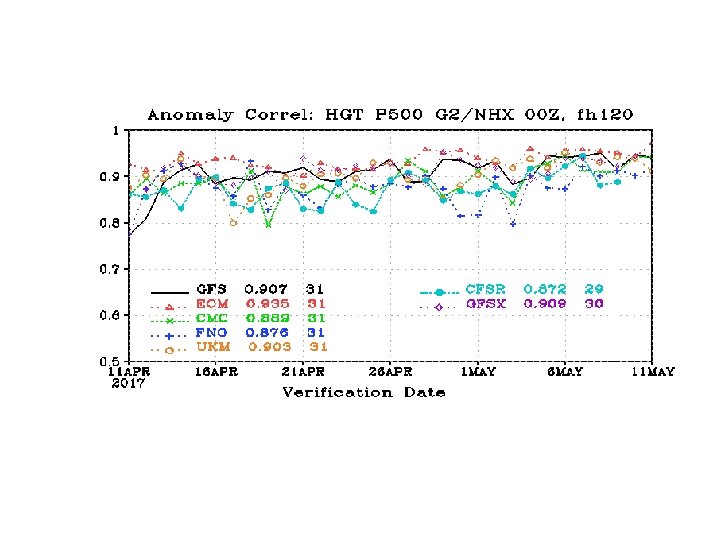
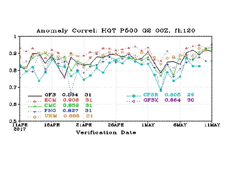
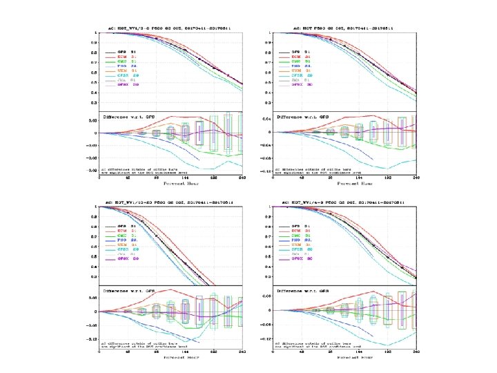
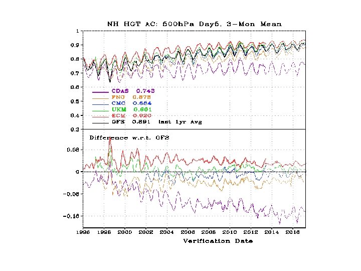
GFS is not the best global model and is not the best

New Global Model: FV 3 developed by NOAA’s GFDL part of the Next Generation Global Prediction System project (NGGPS)

Grid based

Cubed Sphere

Higher Resolution Operational Models

Major U. S. High-Resolution Mesoscale Models (all non-hydrostatic) • WRF-ARW (developed at NCAR) • NMM-B (developed at NCEP Environmental Modeling Center) • COAMPS (U. S. Navy) • MM 5 (NCAR, old, replaced by WRF) • RAMS (Regional Atmospheric Modeling System, Colorado State) • ARPS (Advanced Regional Prediction System): Oklahoma

Operational Mesoscale Model History in US • Early: LFM, NGM (history) • Eta (mainly history) • MM 5: Still used by some, but mainly phased out • NMM- Main NWS mesoscale model, updated Eta model. Sometimes called WRF-NMM and NAM. • WRF-ARW: Heavily used by research and some operational communities. • NMM replaced by NMM-B

NMM-B also called NAM (North American Mesoscale) model • Hybrid sigma-pressure vertical coordinate • 60 levels • Betts-Miller-Janjic convective parameterization scheme • Mellor-Yamada-Janji boundary layer scheme

NMM-B Nests • One-way nested forecasts computed concurrently with the 12 -km NMM-B parent run for – – – CONUS (4 km to 60 hours) Alaska (6 km to 60 hours) Hawaii (3 km to 60 hours) Puerto Rico (3 km to 60 hours) For fire weather, moveable 1. 33 -km CONUS and 1. 5 -km Alaska nests are also run concurrently (to 36 hours). – Call them HRW-High Resolution Windows • A change in horizontal grid from Arakawa. E to Arakawa-B grid, which speeds up computations without degrading the forecast

NMMB 4 -km Conus

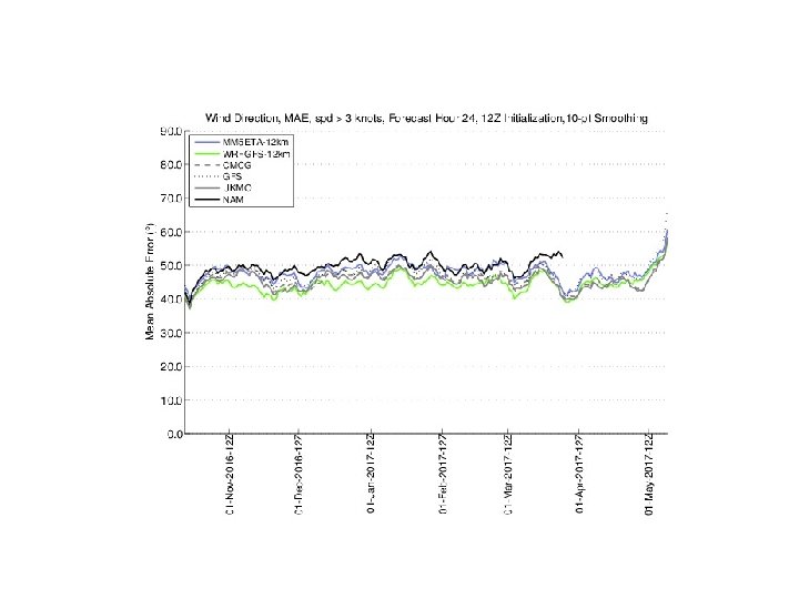
NCEP NAM • Generally less skillful than GFS, even over U. S. • Generally inferior to WRF-ARW at same resolution (more diffusion and smoothing, worse numerics)

Navy COAMPS (Coupled Ocean/Atmosphere Mesoscale Prediction System) • Sigma-Z • Atmosphere and Ocean

http: //www. nrlmry. navy. mil/coa mps-web/home

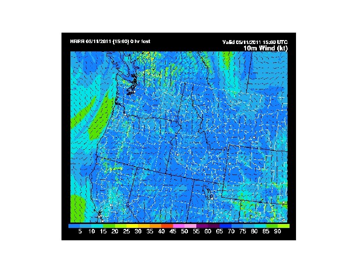
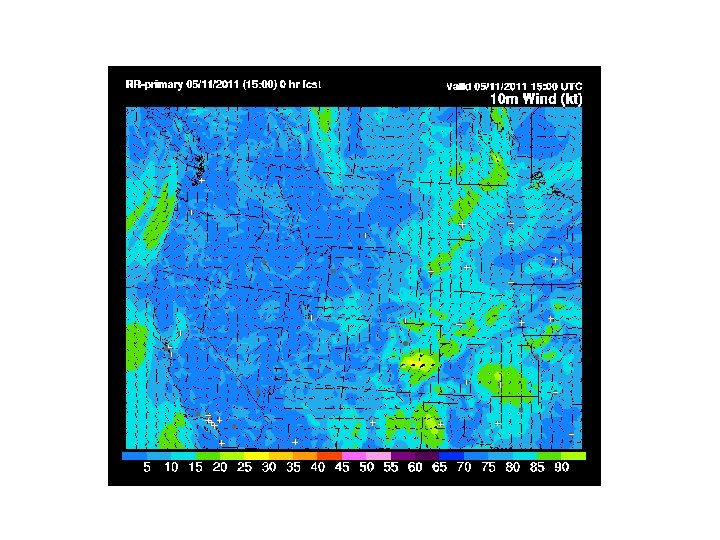
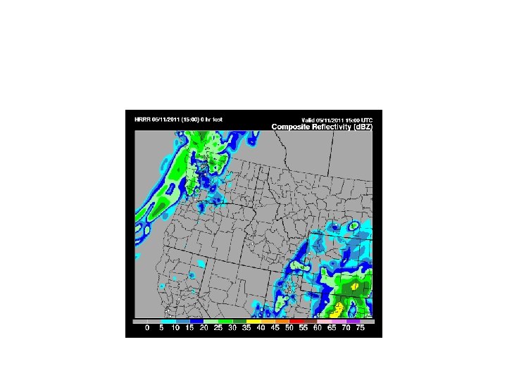
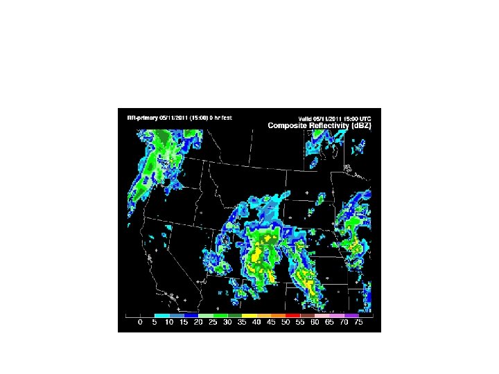
Rapid Refresh NWP A Powerful Tool For Nowcasting Two Resolution: RUC: 13 km HRRR: 3 km

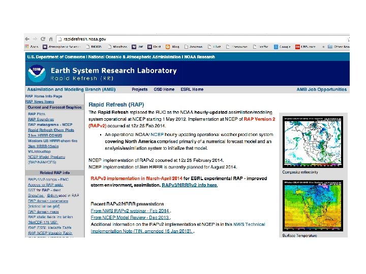
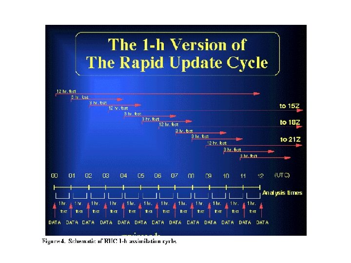
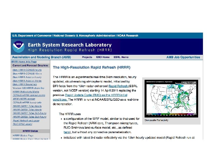
Rapid Refresh (RR). AKA RUC • A major issue is how to assimilate and use the rapidly increasing array of off-time or continuous observations (not a 00 and 12 UTC world anymore! • Want very good analyses and very good short-term forecasts (1 -3 -6 hr) • The RUC/RR ingests and assimilates data hourly, and then makes short-term forecasts • Uses the WRF model…which uses a hybrid sigma/isentropic vertical coordinate • Resolution: Rapid Refresh: 13 km and 50 levels, High Resolution Rapid Refresh (3 km)

Rapid Refresh and HRRR NOAA hourly updated models 13 km Rapid Refresh (RAP) (mesoscale) Version 2 – scheduled NCEP implementation Q 2 (currently 28 Jan) 3 km HRRR (storm-scale) High-Resolution Rapid Refresh RAP HRRR Scheduled NCEP Implementation Q 3 2014 NCEP Production Suite Review Rapid Refresh / HRRR 3 -4 December 2013 82

Observations Used Hourly Observations RAP 2013 N. Amer Rawinsonde (T, V, RH) 120 Profiler – NOAA Network (V) 21 Profiler – 915 MHz (V, Tv) 25 Radar – VAD (V) 125 Radar reflectivity - CONUS 1 km Lightning (proxy reflectivity) NLDN, GLD 360 Aircraft (V, T) 2 -15 K Aircraft - WVSS (RH) 0 -800 Surface/METAR (T, Td, V, ps, cloud, vis, wx) 2200 - 2500 Buoys/ships (V, ps) 200 -400 GOES AMVs (V) 2000 - 4000 AMSU/HIRS/MHS radiances Used GOES cloud-top press/temp 13 km GPS – Precipitable water 260 Wind. Sat scatterometer 2 -10 K

RAPv 2 Hybrid Data Assimilation 14 z 13 z ESRL/GSD RAP 2013 Uses GFS 80 -member ensemble Available four times per day valid at 03 z, 09 z, 15 z, 21 z HM Obs Refl Obs GSI Hybrid GSI HM Anx Digital Filter Obs 1 h r fc st Obs HM Obs Refl Obs 18 hr fcst GSI Hybrid GSI HM Anx Digital Filter 15 z 80 -member GFS En. KF Ensemble forecast valid at 15 Z (9 -hr fcst from 6 Z) Obs 1 h r fc st 13 km RAP Cycle HM Obs Refl Obs 18 hr fcst GSI Hybrid GSI HM Anx Digital Filter 18 hr fcst

Rapid Refresh: 13 km and larger domain

High-Resolution Rapid Refresh: 3 km, 1 hr, smaller domain

http: //www. spc. noaa. gov/exper/hrrr/

Accessing NWP Models • The department web site (go to weather loops or weather discussion) provides easy access to many model forecasts. • The NCEP web site is good place to start for NWS models. http: //www. nco. ncep. noaa. gov/pmb/nwprod/analysis/ • The Department Regional Prediction Page gets to the department regional modeling output. http: //www. atmos. washington. edu/mm 5 rt/

http: //mag. ncep. noaa. gov/

A Palette of Models • Forecasters thus have a palette of model forecasts. • They vary by: – – Region simulated Resolution Model Physics Data used in the assimilation/initialization process • The diversity of models can be a very useful tool to a forecaster.

RTMA (Real Time Mesoscale Analysis System) NWS Mesoscale Analysis System for verifying model output and human forecasts.

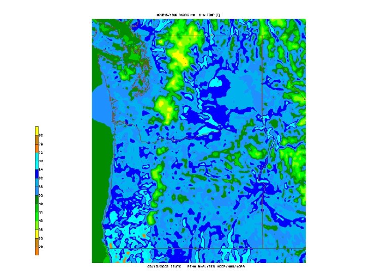
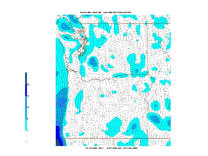
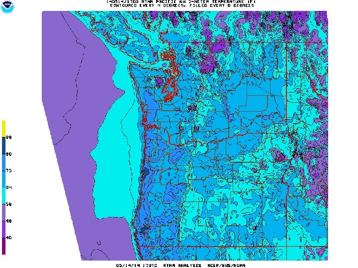
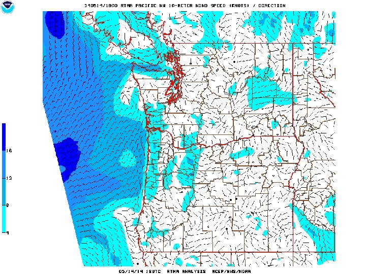
Real-Time Mesoscale Analysis RTMA • Downscales a short-term forecast to fineresolution terrain and coastlines and then uses observations to produce a fine-resolution analysis. • Performs a 2 -dimensional variational analysis (2 d -var) using current surface observations, including mesonets, and scatterometer winds over water, using short-term forecast as first guess. • Provides estimates of the spatially-varying magnitude of analysis errors • Also includes hourly Stage II precipitation estimates and Effective Cloud Amount, a GOES derived product • Either a 5 -km or 2. 5 km analysis.

RTMA • The RTMA depends on a short-term model forecast for a first guess, thus the RTMA is affected by the quality of the model's analysis/forecast system • CONUS first guess is downscaled from a 1 hour RR forecast. • Because the RTMA uses mesonet data, which is of highly variable quality due to variations in sensor siting and sensor maintenance, observation quality control strongly affects the analysis.

Why does NWS want this? • Gridded verification of their gridded forecasts (NDFD) • Serve as a mesoscale Analysis of Record (AOR) • For mesoscale forecasting and studies.

TX 2 m Temperature Analysis 102

The End

WRF and NMM

History of WRF model • An attempt to create a national mesoscale prediction system to be used by both operational and research communities during 1990 s. • A new, state-of-the-art model that would have good conservation characteristics (e. g. , conservation of mass) and good numerics (so not too much numerical diffusion) • A model that could parallelize well on many processors and easy to modify. • Plug-compatible physics to foster improvements in model physics. • Designed for grid spacings of 1 -10 km

NWS goes its own way • ARW (Advanced Research WRF) developed at NCAR • Non-hydrostatic Mesoscale Model (NMM) Core developed at NCEP NMM ARW

The NCAR ARW Core Model: (See: www. wrf-model. org) § Terrain following vertical coordinate § two-way nesting, any ratio § Conserves mass, entropy and scalars using up to 6 th order spatial differencing equ for fluxes. Very good numerics, less implicit smoothing in numerics. § NCAR physics package (converted from MM 5 and Eta), NOAH unified land-surface model, NCEP physics adapted too

NWS 1—Used NMM-B in the NAM RUN • Run every six hours over N. American and adjacent ocean • Run to 84 hours at 12 -km grid spacing. • Uses the Grid-Point Statistical Interpolation (GSI) data assimilation system (3 DVAR) • Start with GDAS (GFS analysis) as initial first guess at t-12 hour (the start of the analysis cycle) • Runs an intermittent data assimilation cycle every three hours until the initialization time. 1 -Non-hydrostatic mesoscale model, NAM: North American Mesoscale run