36ea4866572bc6dadd6e8579ebbdee10.ppt
- Количество слайдов: 76
4. Continuous Random Variables and Probability Distributions Li Jie
4. 1 Continuous random variables and probability density functions Continuous random variables DEFINTION: A random variable X is said to be continuous if its set of possible values is an entire interval of numbers--that is, if for some A<B, any number X between A and B is possible. Li Jie
Example 4. 1: If in the study of the ecology of a lake , we make depth measurements at randomly chosen location, then X=the depth at such a location is a continuous rv. Here A is the minimum depth in the region being sampled, and B is the maximum depth. If the measurement scale of X can be subdivided to any extent desired, then variable is continuous ; if it cannot, the variable is discrete. Li Jie
Probability Distributions for Continuous Variables Suppose the variable X of interest is depth of a lake at a randomly chosen point on the surface, let M=the maximum depth, so that any number in the interval [0, M] is a possible value of X. If we “discretize” X by measuring depth to the nearest meter , then possible value are nonnegative less than or equal to M. the resulting discrete distribution of depth can be pictured using a probability histogram , Li Jie
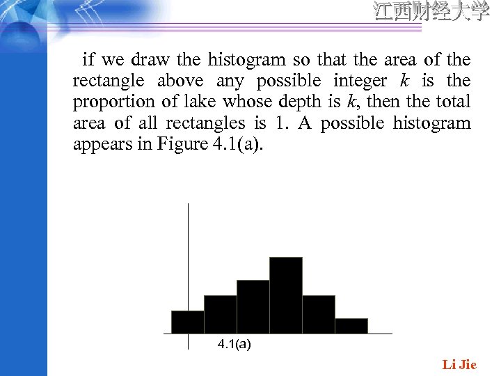
if we draw the histogram so that the area of the rectangle above any possible integer k is the proportion of lake whose depth is k, then the total area of all rectangles is 1. A possible histogram appears in Figure 4. 1(a) Li Jie
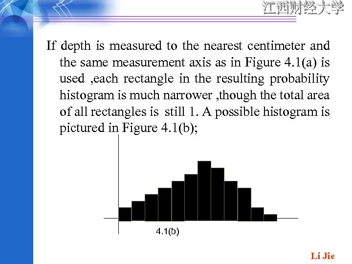
If depth is measured to the nearest centimeter and the same measurement axis as in Figure 4. 1(a) is used , each rectangle in the resulting probability histogram is much narrower , though the total area of all rectangles is still 1. A possible histogram is pictured in Figure 4. 1(b); 4. 1(b) Li Jie
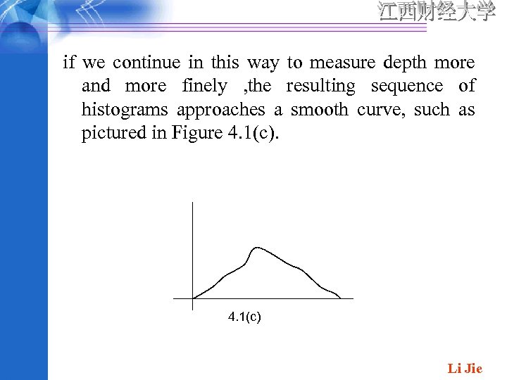
if we continue in this way to measure depth more and more finely , the resulting sequence of histograms approaches a smooth curve, such as pictured in Figure 4. 1(c) Li Jie
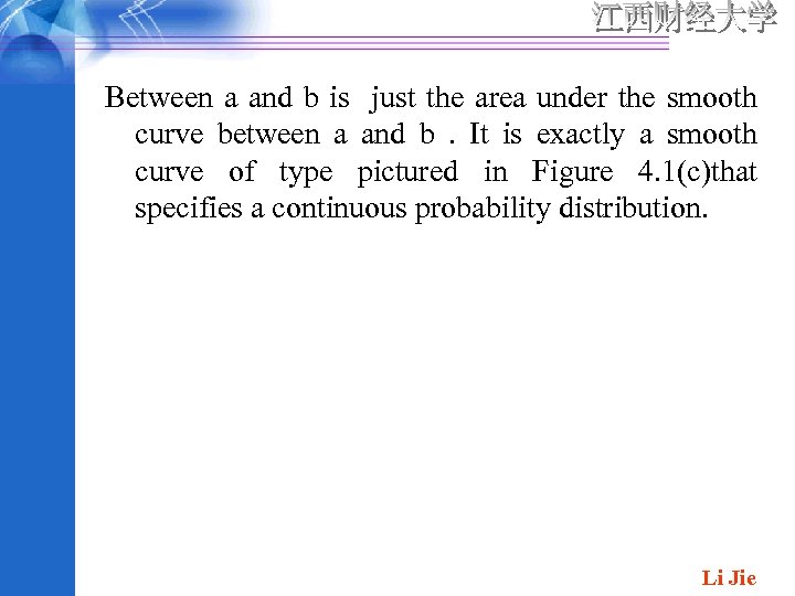
Between a and b is just the area under the smooth curve between a and b. It is exactly a smooth curve of type pictured in Figure 4. 1(c)that specifies a continuous probability distribution. Li Jie
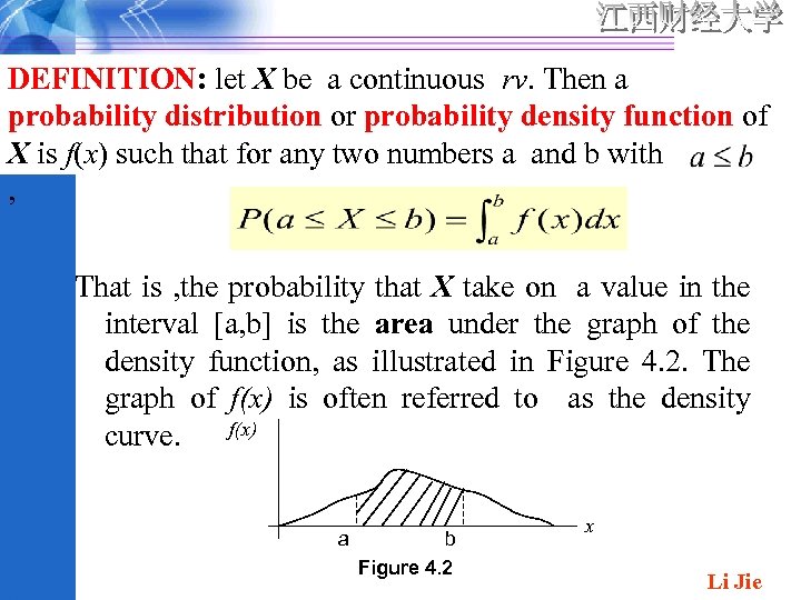
DEFINITION: let X be a continuous rv. Then a probability distribution or probability density function of X is f(x) such that for any two numbers a and b with , That is , the probability that X take on a value in the interval [a, b] is the area under the graph of the density function, as illustrated in Figure 4. 2. The graph of f(x) is often referred to as the density f(x) curve. a b Figure 4. 2 x Li Jie
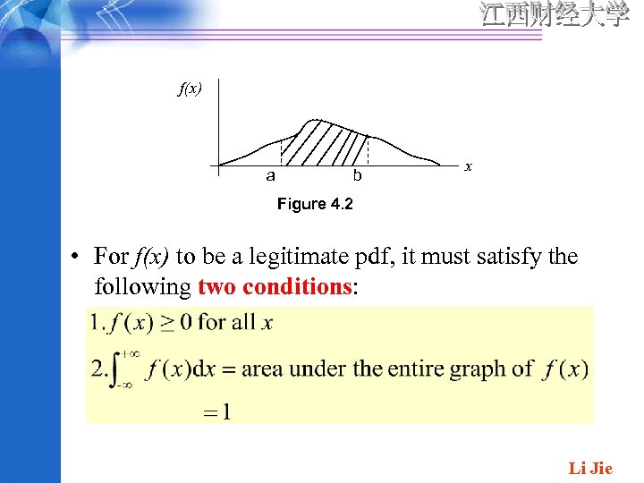
f(x) a b x Figure 4. 2 • For f(x) to be a legitimate pdf, it must satisfy the following two conditions: Li Jie
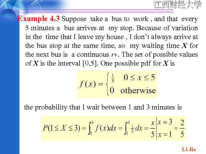
Example 4. 3 Suppose take a bus to work , and that every 5 minutes a bus arrives at my stop. Because of variation in the time that I leave my house , I don’t always arrive at the bus stop at the same time, so my waiting time X for the next bus is a continuous rv. The set of possible values of X is the interval [0, 5]. One possible pdf for X is the probability that I wait between 1 and 3 minutes is Li Jie
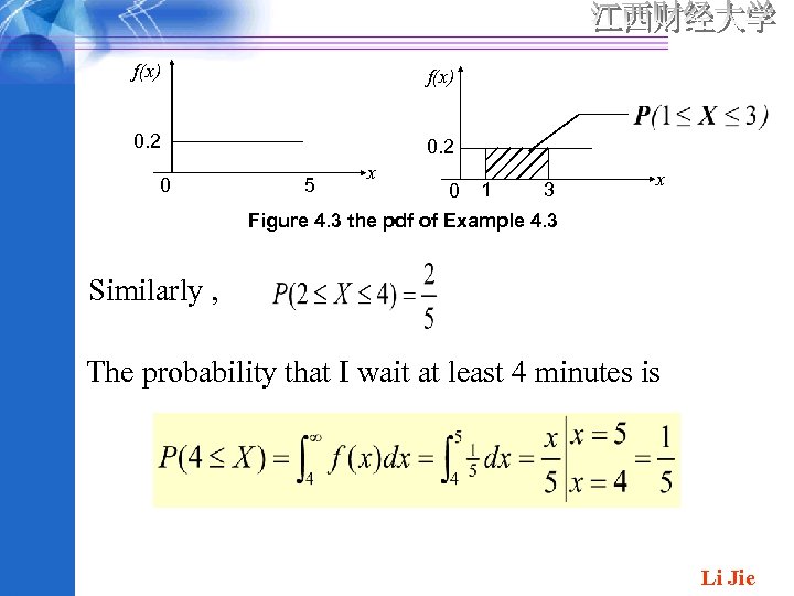
f(x) 0. 2 0 5 x 3 0 1 Figure 4. 3 the pdf of Example 4. 3 x Similarly , The probability that I wait at least 4 minutes is Li Jie
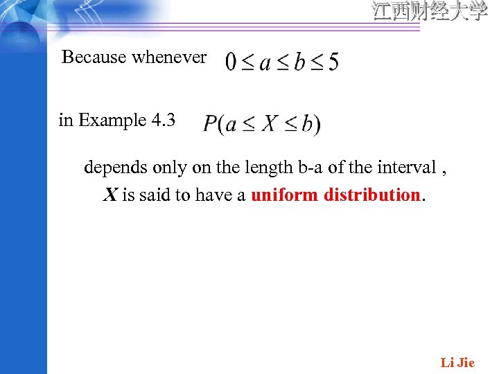
Because whenever in Example 4. 3 depends only on the length b-a of the interval , X is said to have a uniform distribution. Li Jie
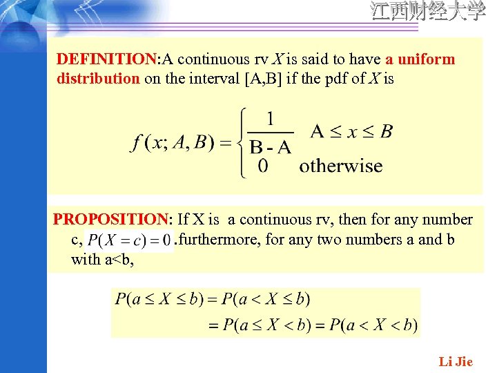
DEFINITION: A continuous rv X is said to have a uniform distribution on the interval [A, B] if the pdf of X is PROPOSITION: If X is a continuous rv, then for any number c, . furthermore, for any two numbers a and b with a<b, Li Jie
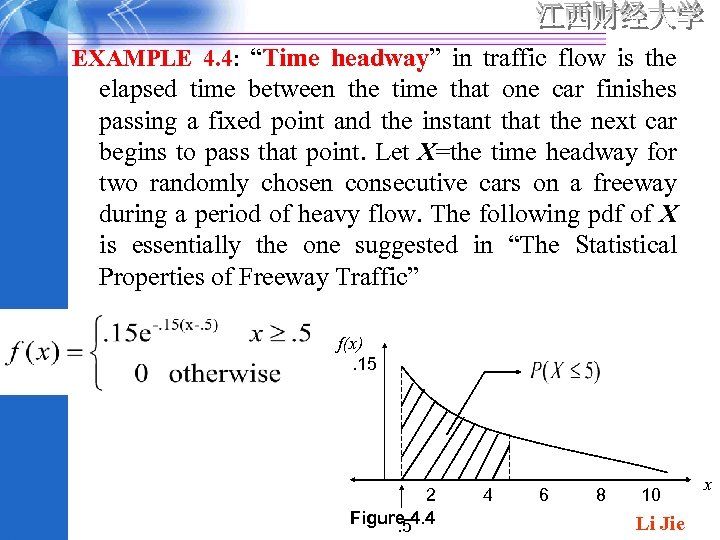
EXAMPLE 4. 4: “Time headway” in traffic flow is the elapsed time between the time that one car finishes passing a fixed point and the instant that the next car begins to pass that point. Let X=the time headway for two randomly chosen consecutive cars on a freeway during a period of heavy flow. The following pdf of X is essentially the one suggested in “The Statistical Properties of Freeway Traffic” f(x). 15 2 Figure 4. 4. 5 4 6 8 10 Li Jie x
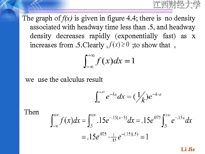
The graph of f(x) is given in figure 4. 4; there is no density associated with headway time less than. 5, and headway density decreases rapidly (exponentially fast) as x increases from. 5. Clearly , ; to show that , we use the calculus result Then Li Jie
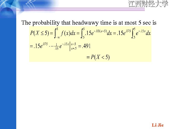
The probability that headwawy time is at most 5 sec is Li Jie
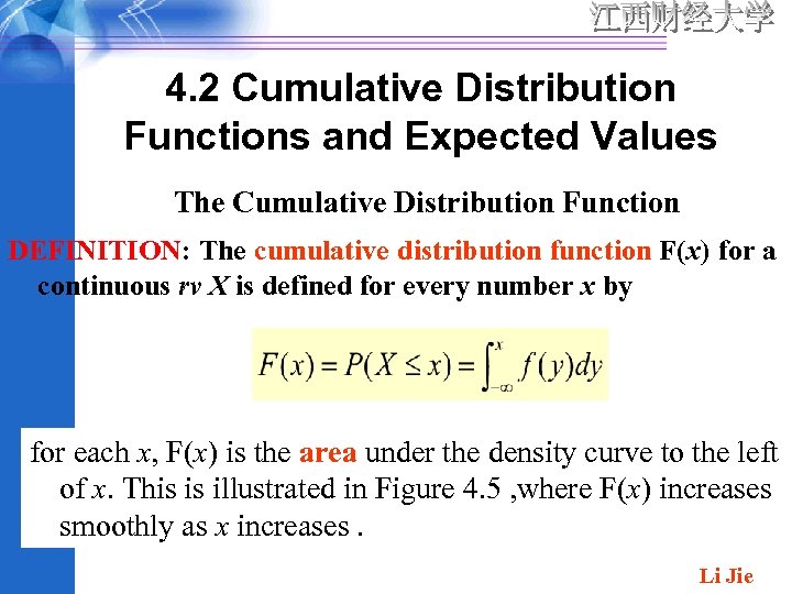
4. 2 Cumulative Distribution Functions and Expected Values The Cumulative Distribution Function DEFINITION: The cumulative distribution function F(x) for a continuous rv X is defined for every number x by for each x, F(x) is the area under the density curve to the left of x. This is illustrated in Figure 4. 5 , where F(x) increases smoothly as x increases. Li Jie
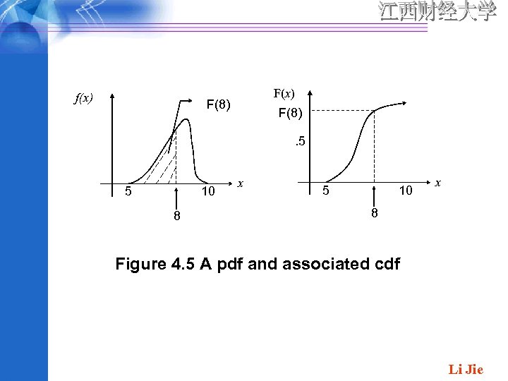
f(x) F(8). 5 5 10 8 x 5 10 x 8 Figure 4. 5 A pdf and associated cdf Li Jie
![Example 4. 5 : Let X have a uniform distribution on [A, B]. The Example 4. 5 : Let X have a uniform distribution on [A, B]. The](https://present5.com/presentation/36ea4866572bc6dadd6e8579ebbdee10/image-20.jpg)
Example 4. 5 : Let X have a uniform distribution on [A, B]. The density function is show in Figure 4. 6. For x<A , F(x)=0 , since there is no area under the graph of the density function to the left of such an x. f(x) A B x A x B Figure 4. 6 The pdf for a uniform distribution Finally , for , Li Jie
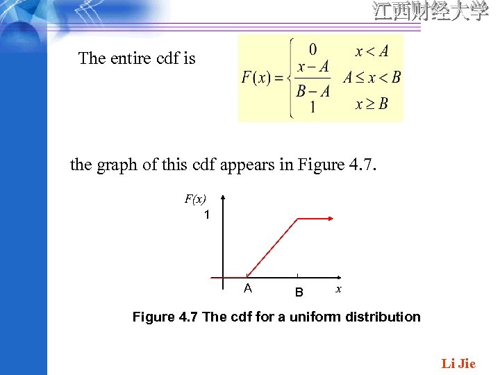
The entire cdf is the graph of this cdf appears in Figure 4. 7. F(x) 1 A B x Figure 4. 7 The cdf for a uniform distribution Li Jie
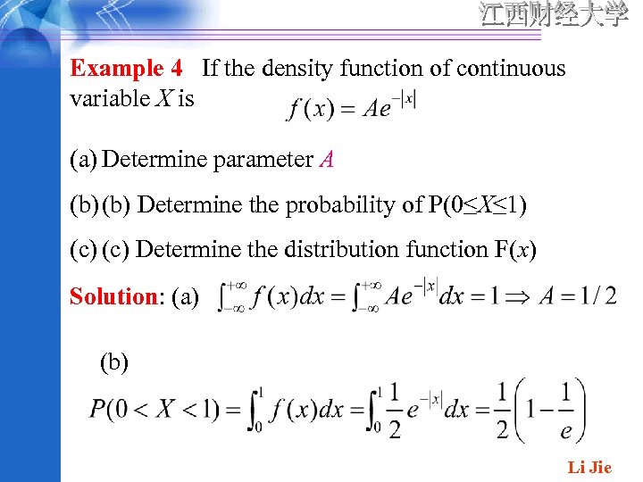
Example 4 If the density function of continuous variable X is (a) Determine parameter A (b) Determine the probability of P(0≤X≤ 1) (c) Determine the distribution function F(x) Solution: (a) (b) Li Jie
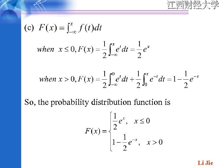
(c) So, the probability distribution function is Li Jie
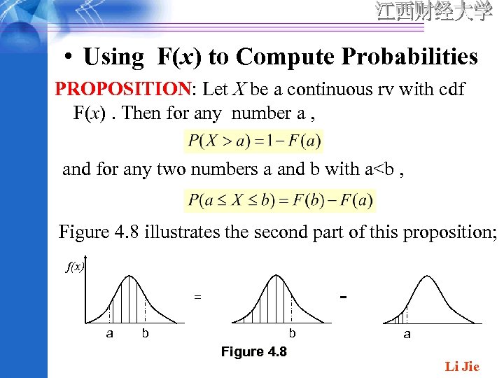
• Using F(x) to Compute Probabilities PROPOSITION: Let X be a continuous rv with cdf F(x). Then for any number a , and for any two numbers a and b with a<b , Figure 4. 8 illustrates the second part of this proposition; f(x) - = a b b Figure 4. 8 a Li Jie
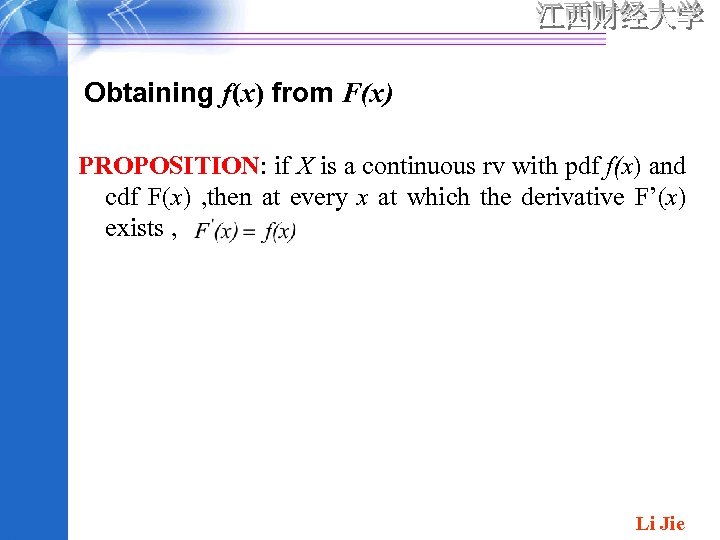
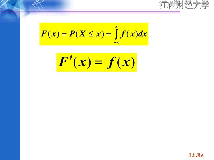
Obtaining f(x) from F(x) PROPOSITION: if X is a continuous rv with pdf f(x) and cdf F(x) , then at every x at which the derivative F’(x) exists , Li Jie
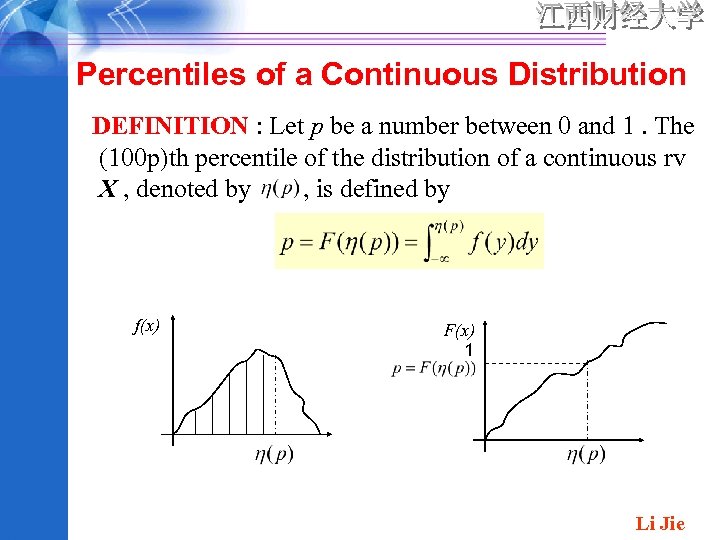
Percentiles of a Continuous Distribution DEFINITION : Let p be a number between 0 and 1. The (100 p)th percentile of the distribution of a continuous rv X , denoted by , is defined by f(x) F(x) 1 Li Jie
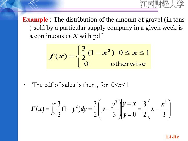
Example : The distribution of the amount of gravel (in tons ) sold by a particular supply company in a given week is a continuous rv X with pdf • The cdf of sales is then , for 0<x<1 Li Jie
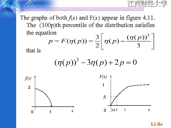
The graphs of both f(x) and F(x) appear in figure 4. 11. The (100 p)th percentile of the distribution satisfies the equation that is f(x) F(x) 2 1. 5 0 1 x 0. 347 1 x Li Jie
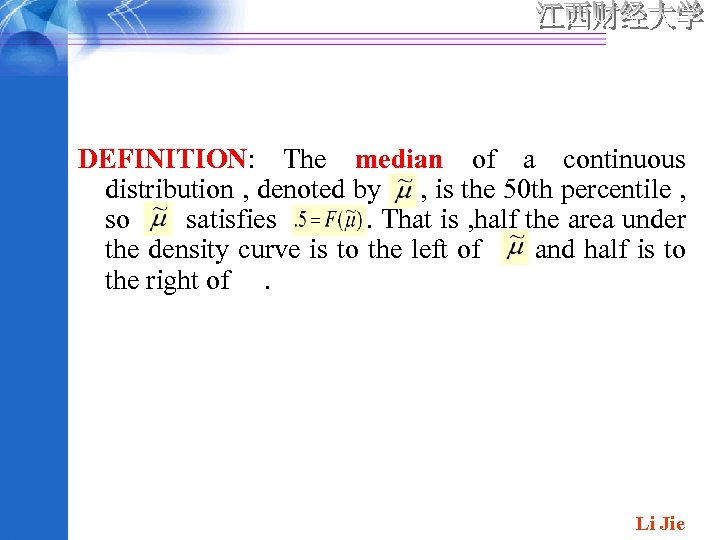
DEFINITION: The median of a continuous distribution , denoted by , is the 50 th percentile , so satisfies. That is , half the area under the density curve is to the left of and half is to the right of. Li Jie
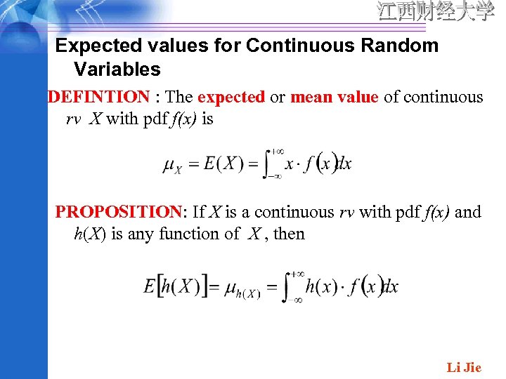
Expected values for Continuous Random Variables DEFINTION : The expected or mean value of continuous rv X with pdf f(x) is PROPOSITION: If X is a continuous rv with pdf f(x) and h(X) is any function of X , then Li Jie
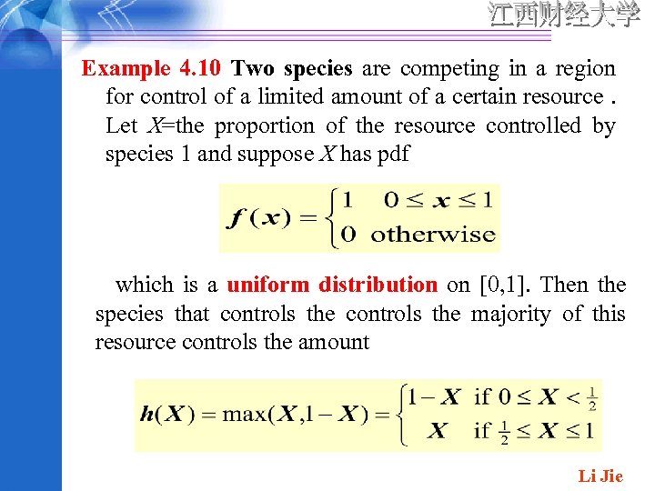
Example 4. 10 Two species are competing in a region for control of a limited amount of a certain resource. Let X=the proportion of the resource controlled by species 1 and suppose X has pdf which is a uniform distribution on [0, 1]. Then the species that controls the majority of this resource controls the amount Li Jie
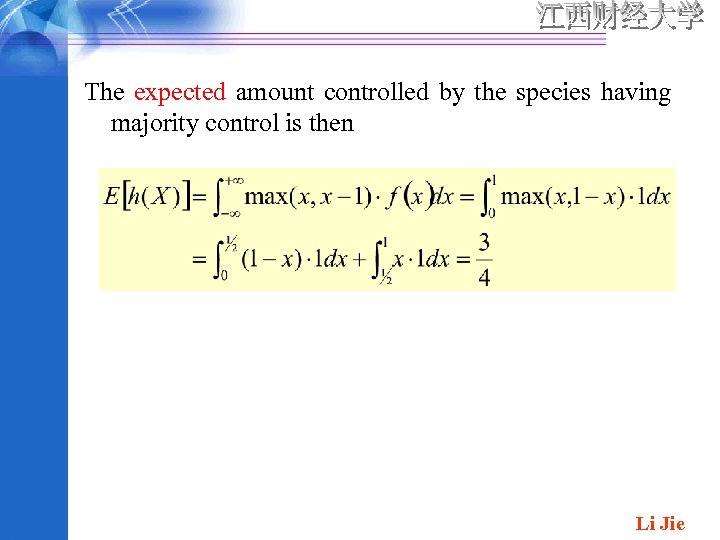
The expected amount controlled by the species having majority control is then Li Jie
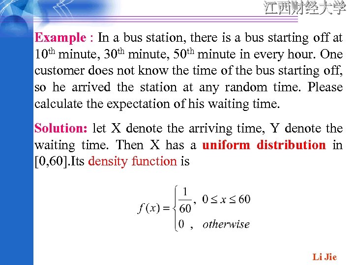
Example : In a bus station, there is a bus starting off at 10 th minute, 30 th minute, 50 th minute in every hour. One customer does not know the time of the bus starting off, so he arrived the station at any random time. Please calculate the expectation of his waiting time. Solution: let X denote the arriving time, Y denote the waiting time. Then X has a uniform distribution in [0, 60]. Its density function is Li Jie
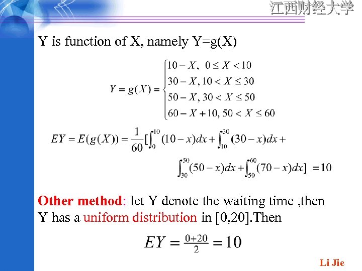
Y is function of X, namely Y=g(X) Other method: let Y denote the waiting time , then Y has a uniform distribution in [0, 20]. Then Li Jie
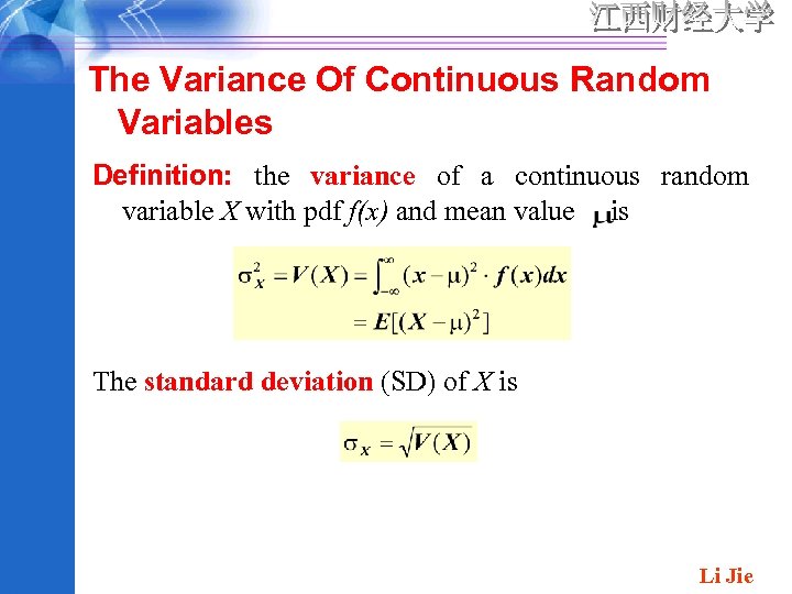
The Variance Of Continuous Random Variables Definition: the variance of a continuous random variable X with pdf f(x) and mean value is The standard deviation (SD) of X is Li Jie
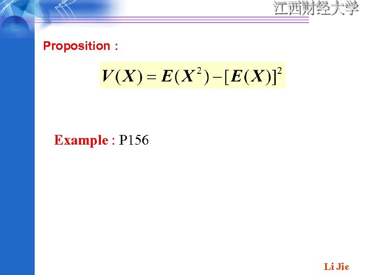
Proposition : Example : P 156 Li Jie
4. 3 The Normal Distribution Li Jie
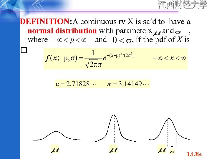
DEFINITION: A continuous rv X is said to have a normal distribution with parameters and , where and , if the pdf of X is Li Jie

u. S y m m u. B etr ell ic sh ap ed paramt er, is the standar u. The d left density deviatio portio in two n and is n of ends of called the the curve distributi scale is on the parame mirro function ter. r Hence is low. It denote image increases X ~ N ( of the towards , ). right the portio middle n of the distributi Li Jie
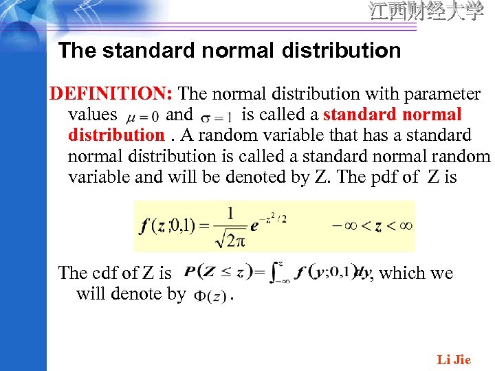
The standard normal distribution DEFINITION: The normal distribution with parameter values and is called a standard normal distribution. A random variable that has a standard normal distribution is called a standard normal random variable and will be denoted by Z. The pdf of Z is The cdf of Z is will denote by . , which we Li Jie
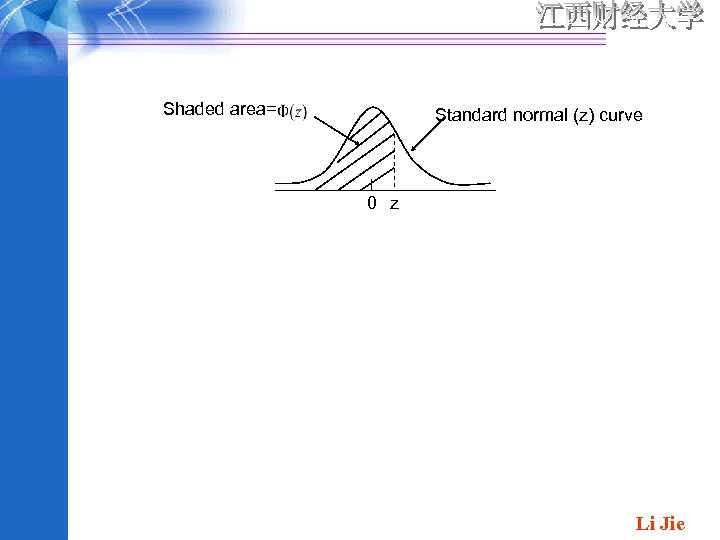
Shaded area= Standard normal (z) curve 0 z Li Jie
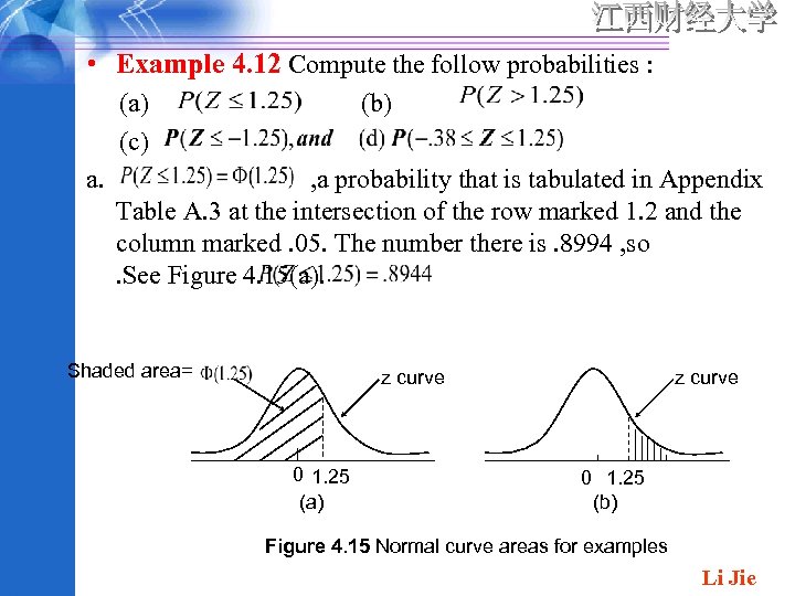
• Example 4. 12 Compute the follow probabilities : (a) (c) a. (b) , a probability that is tabulated in Appendix Table A. 3 at the intersection of the row marked 1. 2 and the column marked. 05. The number there is. 8994 , so. See Figure 4. 15(a). Shaded area= z curve 0 1. 25 (a) z curve 0 1. 25 (b) Figure 4. 15 Normal curve areas for examples Li Jie
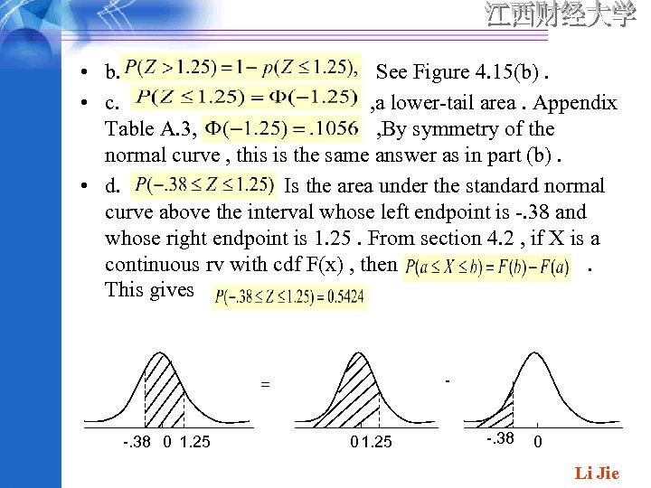
• b. See Figure 4. 15(b). • c. , a lower-tail area. Appendix Table A. 3, , By symmetry of the normal curve , this is the same answer as in part (b). • d. Is the area under the standard normal curve above the interval whose left endpoint is -. 38 and whose right endpoint is 1. 25. From section 4. 2 , if X is a continuous rv with cdf F(x) , then. This gives. - = -. 38 0 1. 25 -. 38 0 Li Jie
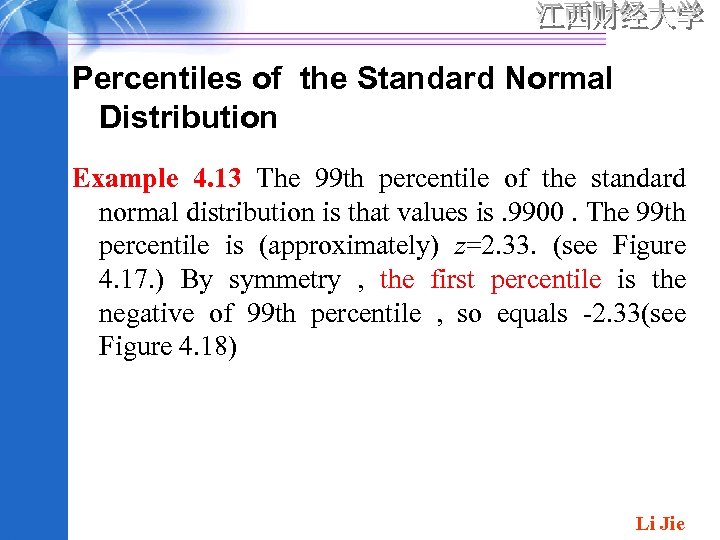
Percentiles of the Standard Normal Distribution Example 4. 13 The 99 th percentile of the standard normal distribution is that values is. 9900. The 99 th percentile is (approximately) z=2. 33. (see Figure 4. 17. ) By symmetry , the first percentile is the negative of 99 th percentile , so equals -2. 33(see Figure 4. 18) Li Jie
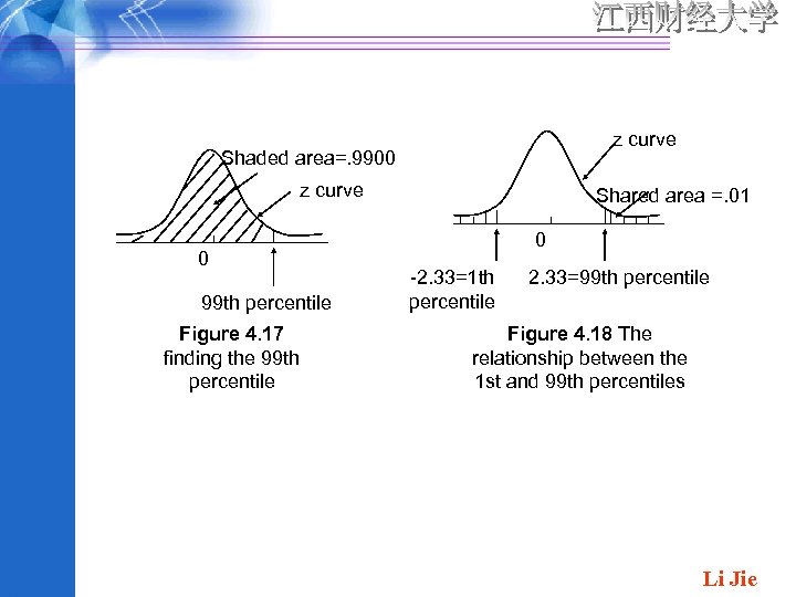
z curve Shaded area=. 9900 z curve 0 99 th percentile Figure 4. 17 finding the 99 th percentile Shared area =. 01 0 -2. 33=1 th percentile 2. 33=99 th percentile Figure 4. 18 The relationship between the 1 st and 99 th percentiles Li Jie
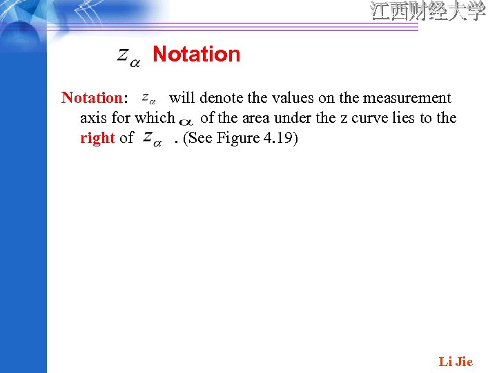
Notation: will denote the values on the measurement axis for which of the area under the z curve lies to the right of. (See Figure 4. 19) Li Jie
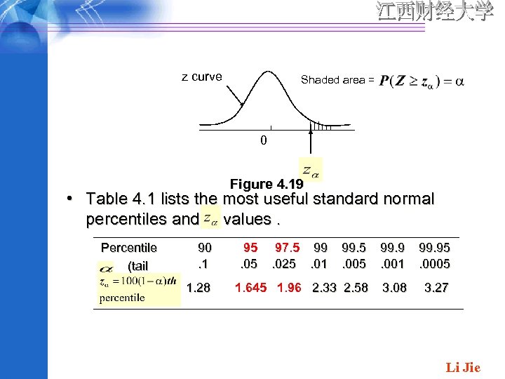
z curve Shaded area = 0 Figure 4. 19 • Table 4. 1 lists the most useful standard normal percentiles and values. Percentile (tail area) 90 95 97. 5 99. 95 90 . 1 . 05 . 025 . 01 . 005 . 001 . 0005 1. 28 1. 645 1. 96 2. 33 2. 58 3. 08 3. 27 1. 28 Li Jie
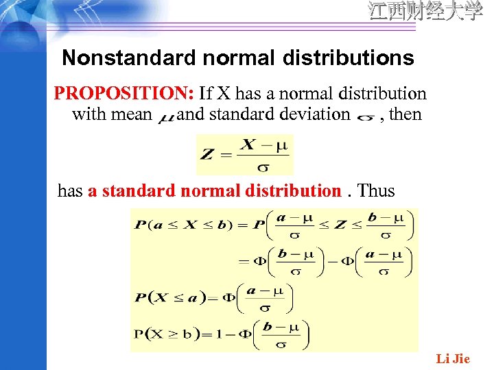
Nonstandard normal distributions PROPOSITION: If X has a normal distribution with mean and standard deviation , then has a standard normal distribution. Thus Li Jie
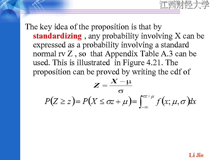
The key idea of the proposition is that by standardizing , any probability involving X can be expressed as a probability involving a standard normal rv Z , so that Appendix Table A. 3 can be used. This is illustrated in Figure 4. 21. The proposition can be proved by writing the cdf of Li Jie
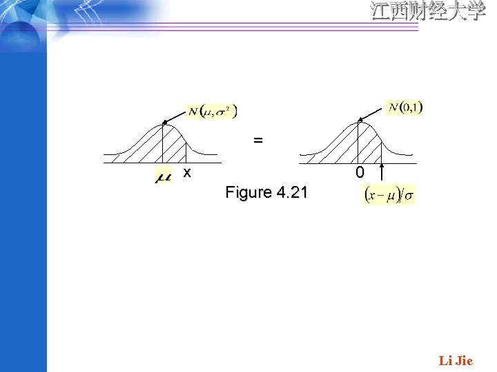
= x 0 Figure 4. 21 Li Jie
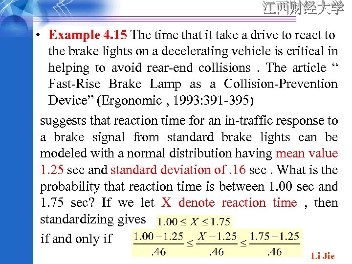
• Example 4. 15 The time that it take a drive to react to the brake lights on a decelerating vehicle is critical in helping to avoid rear-end collisions. The article “ Fast-Rise Brake Lamp as a Collision-Prevention Device” (Ergonomic , 1993: 391 -395) suggests that reaction time for an in-traffic response to a brake signal from standard brake lights can be modeled with a normal distribution having mean value 1. 25 sec and standard deviation of. 16 sec. What is the probability that reaction time is between 1. 00 sec and 1. 75 sec? If we let X denote reaction time , then standardizing gives if and only if Li Jie
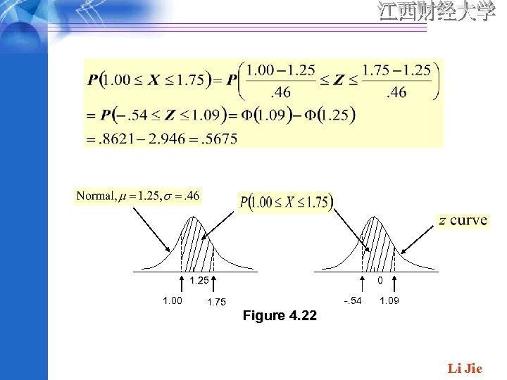
1. 25 1. 00 1. 75 0 -. 54 1. 09 Figure 4. 22 Li Jie
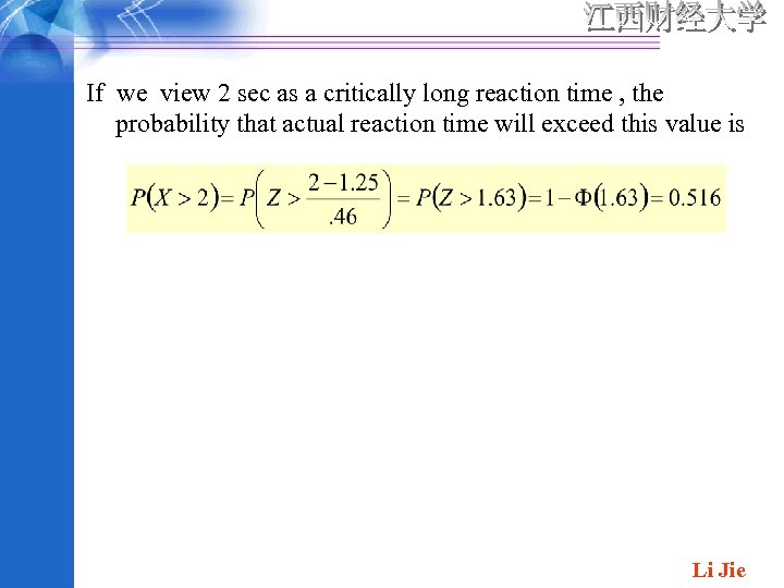
If we view 2 sec as a critically long reaction time , the probability that actual reaction time will exceed this value is Li Jie
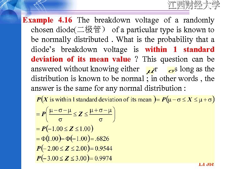
Example 4. 16 The breakdown voltage of a randomly chosen diode(二极管) of a particular type is known to be normally distributed. What is the probability that a diode’s breakdown voltage is within 1 standard deviation of its mean value ? This question can be answered without knowing either or , as long as the distribution is known to be normal ; in other words , the answer is the same for any normal distribution : Li Jie
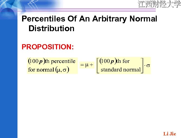
Percentiles Of An Arbitrary Normal Distribution PROPOSITION: Li Jie
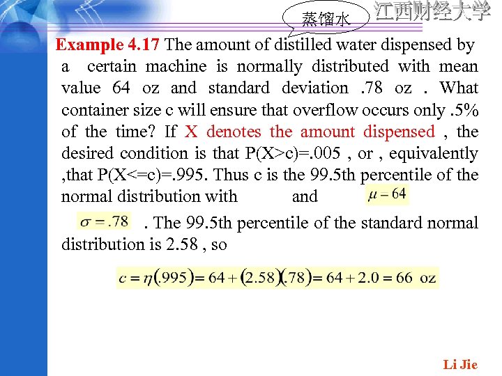
蒸馏水 Example 4. 17 The amount of distilled water dispensed by a certain machine is normally distributed with mean value 64 oz and standard deviation. 78 oz. What container size c will ensure that overflow occurs only. 5% of the time? If X denotes the amount dispensed , the desired condition is that P(X>c)=. 005 , or , equivalently , that P(X<=c)=. 995. Thus c is the 99. 5 th percentile of the normal distribution with and. The 99. 5 th percentile of the standard normal distribution is 2. 58 , so Li Jie
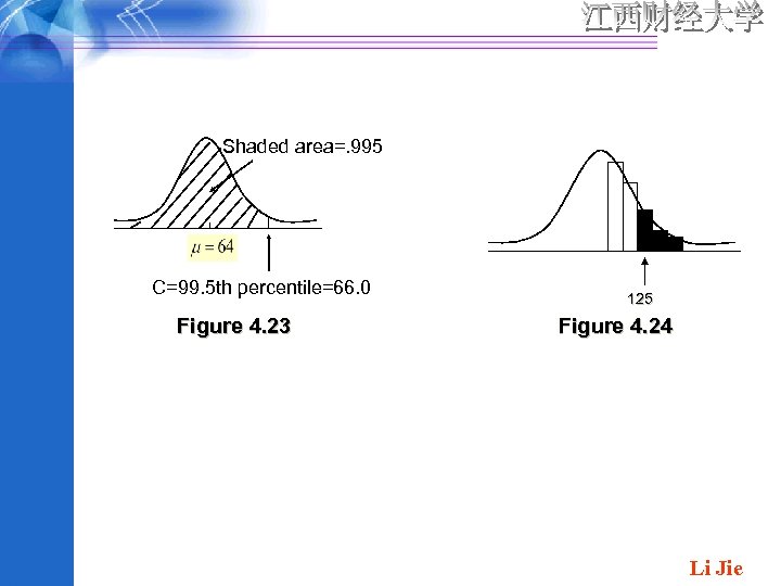
Shaded area=. 995 C=99. 5 th percentile=66. 0 Figure 4. 23 125 Figure 4. 24 Li Jie
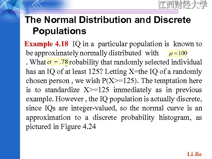
The Normal Distribution and Discrete Populations Example 4. 18 IQ in a particular population is known to be approximately normally distributed with and. What is the probability that randomly selected individual has an IQ of at least 125? Letting X=the IQ of a randomly chosen person , we wish P(X>=125). The temptation here is to standardize X>=125 immediately as in previous example. However , the IQ population is actually discrete, since IQs are integer-valued, so the normal curve is an approximation to a discrete probability histogram, as pictured in Figure 4. 24 Li Jie
• The correction for discreteness of the underlying distribution in Example 4. 18 is often called a continuity correction. It is useful in the following application of the normal distribution to the computation of binomial probabilities. Li Jie
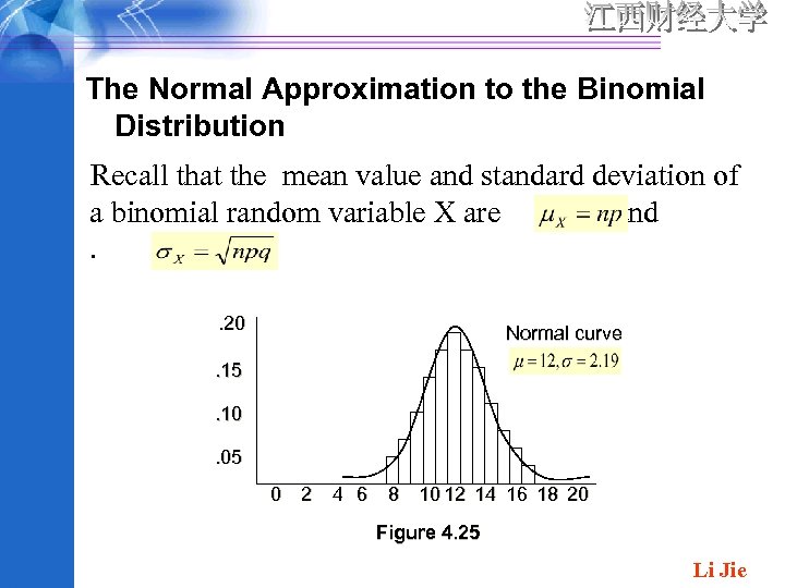
The Normal Approximation to the Binomial Distribution Recall that the mean value and standard deviation of a binomial random variable X are and. . 20 Normal curve . 15. 10. 05 0 2 4 6 8 10 12 14 16 18 20 Figure 4. 25 Li Jie
• More generally, as long as the binomial probability histogram is not too skewed binomial probabilities can be well approximated by normal curve areas. It is then customary to say that X has approximately a normal distribution. Li Jie
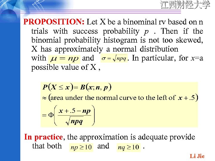
PROPOSITION: Let X be a binominal rv based on n trials with success probability p. Then if the binomial probability histogram is not too skewed, X has approximately a normal distribution with and. In particular, for x=a possible value of X , In practice, the approximation is adequate provide that both and. Li Jie
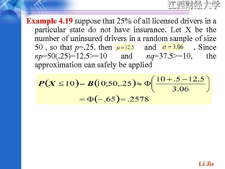
Example 4. 19 suppose that 25% of all licensed drivers in a particular state do not have insurance. Let X be the number of uninsured drivers in a random sample of size 50 , so that p=. 25. then and. Since np=50(. 25)=12. 5>=10 and nq=37. 5>=10, the approximation can safely be applied Li Jie
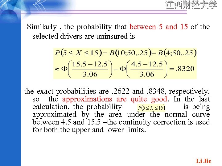
Similarly , the probability that between 5 and 15 of the selected drivers are uninsured is the exact probabilities are. 2622 and. 8348, respectively, so the approximations are quite good. In the last calculation, the probability is being approximated by the area under the normal curve between 4. 5 and 15. 5 –the continuity correction is used for both the upper and lower limits. Li Jie
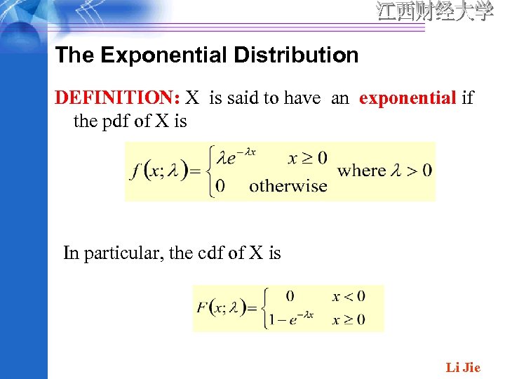
The Exponential Distribution DEFINITION: X is said to have an exponential if the pdf of X is In particular, the cdf of X is Li Jie
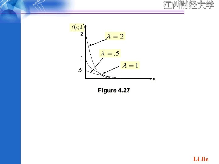
2 1. 5 x Figure 4. 27 Li Jie
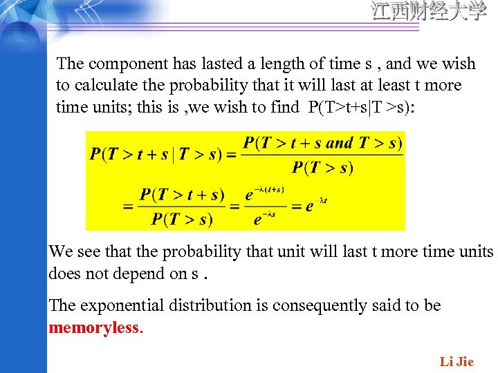
The component has lasted a length of time s , and we wish to calculate the probability that it will last at least t more time units; this is , we wish to find P(T>t+s|T >s): We see that the probability that unit will last t more time units does not depend on s. The exponential distribution is consequently said to be memoryless. Li Jie

Expected values for The Exponential Distribution Li Jie
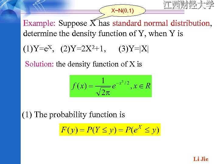
X~N(0, 1) Example: Suppose X has standard normal distribution, determine the density function of Y, when Y is (1)Y=e. X, (2)Y=2 X 2+1, (3)Y=|X| Solution: the density function of X is (1) The probability function is Li Jie
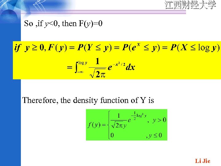
So , if y<0, then F(y)=0 Therefore, the density function of Y is Li Jie
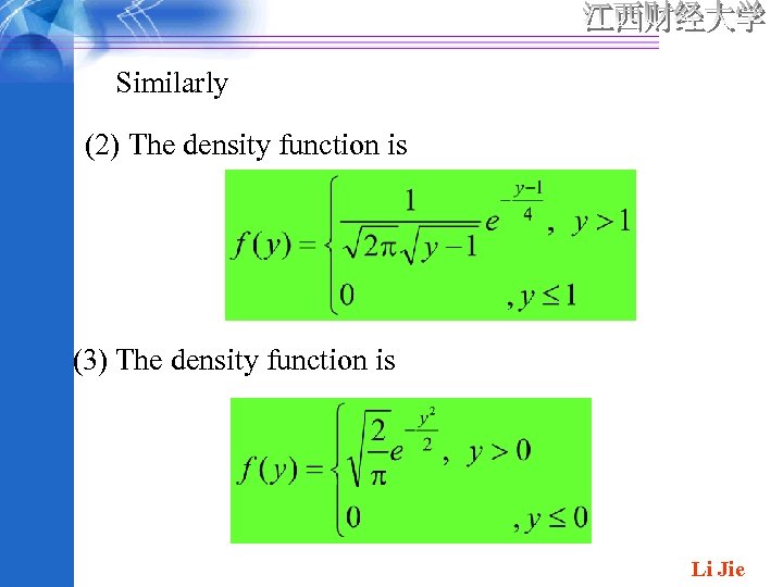
Similarly (2) The density function is (3) The density function is Li Jie
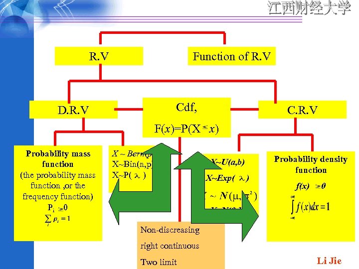
R. V Function of R. V Cdf, D. R. V C. R. V F(x)=P(X x) Probability mass function (the probability mass function , or the frequency function) Pi 0 X ~ Bern(p) X~Bin(n, p) X~P( ) Probability density function X~U(a, b) X~Exp( X~N( , ) ) f(x) 0 X~N(0, 1) Non-discreasing right continuous Two limit Li Jie
Li Jie
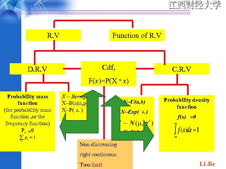
R. V Function of R. V Cdf, D. R. V C. R. V F(x)=P(X x) Probability mass function (the probability mass function , or the frequency function) Pi 0 X ~ Bern(p) X~Bin(n, p) X~P( ) Probability density function X~U(a, b) X~Exp( X~N( , ) ) f(x) 0 X~N(0, 1) Non-discreasing right continuous Two limit Li Jie
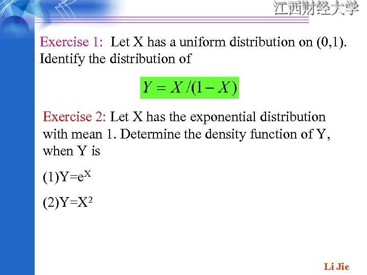
Exercise 1: Let X has a uniform distribution on (0, 1). Identify the distribution of Exercise 2: Let X has the exponential distribution with mean 1. Determine the density function of Y, when Y is (1)Y=e. X (2)Y=X 2 Li Jie

Li Jie
36ea4866572bc6dadd6e8579ebbdee10.ppt