66a0e8157fc21d0d5acc71e87a0d9a0a.ppt
- Количество слайдов: 49
 3 ESO Mathematics A 8 Linear and real-life graphs 1 of 49 © Boardworks Ltd 2005
 Contents A 8 Linear and real-life graphs A 8. 1 Linear graphs A 8. 2 Gradients and intercepts A 8. 3 Parallel and perpendicular lines A 8. 4 Interpreting real-life graphs A 8. 5 Distance-time graphs A 8. 6 Speed-time graphs 2 of 49 © Boardworks Ltd 2005
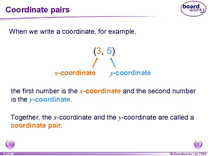 Coordinate pairs When we write a coordinate, for example, (3, 5) x-coordinate y-coordinate the first number is called the x-coordinate and the second number is the y-coordinate. number is called the y-coordinate. Together, the x-coordinate and the y-coordinate are called a coordinate pair. 3 of 49 © Boardworks Ltd 2005
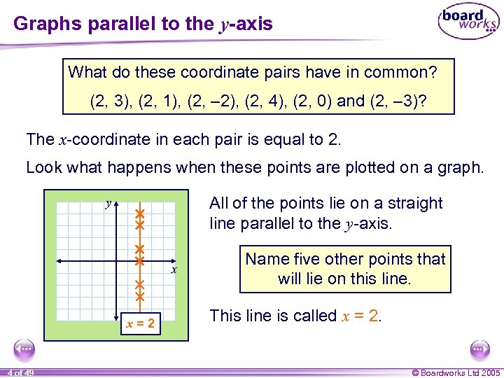 Graphs parallel to the y-axis What do these coordinate pairs have in common? (2, 3), (2, 1), (2, – 2), (2, 4), (2, 0) and (2, – 3)? The x-coordinate in each pair is equal to 2. Look what happens when these points are plotted on a graph. All of the points lie on a straight line parallel to the y-axis. y x x=2 4 of 49 Name five other points that will lie on this line. This line is called x = 2. © Boardworks Ltd 2005
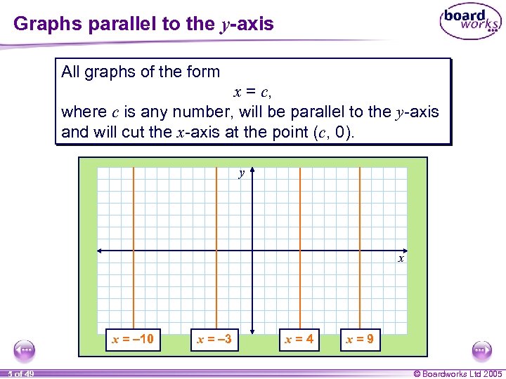 Graphs parallel to the y-axis All graphs of the form x = c, where c is any number, will be parallel to the y-axis and will cut the x-axis at the point (c, 0). y x x = – 10 5 of 49 x = – 3 x=4 x=9 © Boardworks Ltd 2005
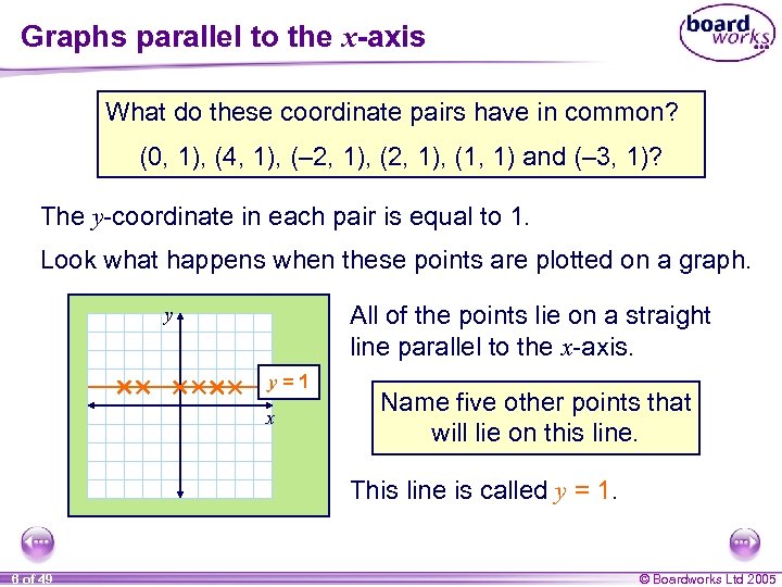 Graphs parallel to the x-axis What do these coordinate pairs have in common? (0, 1), (4, 1), (– 2, 1), (1, 1) and (– 3, 1)? The y-coordinate in each pair is equal to 1. Look what happens when these points are plotted on a graph. All of the points lie on a straight line parallel to the x-axis. y y=1 x Name five other points that will lie on this line. This line is called y = 1. 6 of 49 © Boardworks Ltd 2005
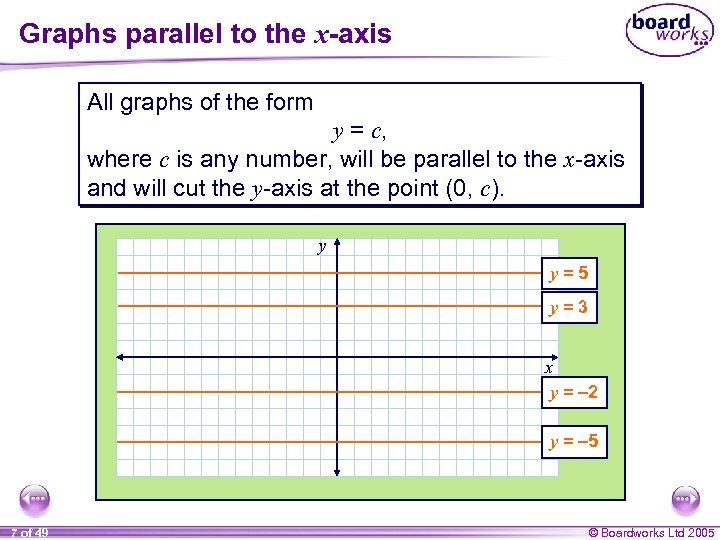 Graphs parallel to the x-axis All graphs of the form y = c, where c is any number, will be parallel to the x-axis and will cut the y-axis at the point (0, c). y y=5 y=3 x y = – 2 y = – 5 7 of 49 © Boardworks Ltd 2005
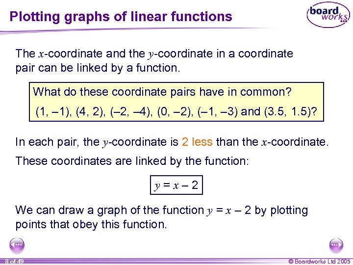 Plotting graphs of linear functions The x-coordinate and the y-coordinate in a coordinate pair can be linked by a function. What do these coordinate pairs have in common? (1, – 1), (4, 2), (– 2, – 4), (0, – 2), (– 1, – 3) and (3. 5, 1. 5)? In each pair, the y-coordinate is 2 less than the x-coordinate. These coordinates are linked by the function: y=x– 2 We can draw a graph of the function y = x – 2 by plotting points that obey this function. 8 of 49 © Boardworks Ltd 2005
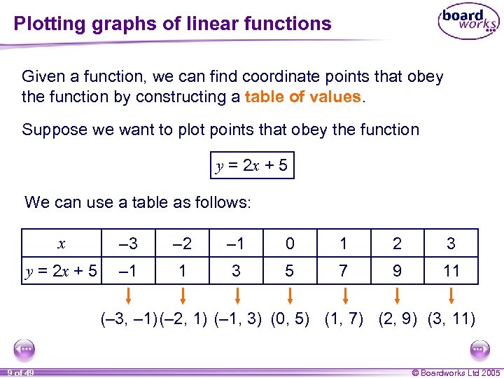 Plotting graphs of linear functions Given a function, we can find coordinate points that obey the function by constructing a table of values. Suppose we want to plot points that obey the function y = 2 x + 5 We can use a table as follows: x – 3 – 2 – 1 0 1 2 3 y = 2 x + 5 – 1 1 3 5 7 9 11 (– 3, – 1) (– 2, 1) (– 1, 3) (0, 5) (1, 7) (2, 9) (3, 11) 9 of 49 © Boardworks Ltd 2005
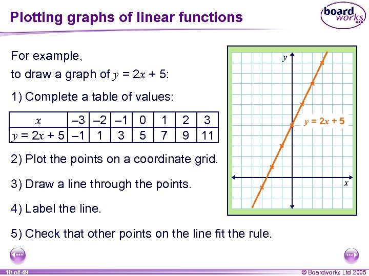 Plotting graphs of linear functions For example, to draw a graph of y = 2 x + 5: y 1) Complete a table of values: x – 3 – 2 – 1 0 y = 2 x + 5 – 1 1 3 5 1 7 2 3 9 11 y = 2 x + 5 2) Plot the points on a coordinate grid. 3) Draw a line through the points. x 4) Label the line. 5) Check that other points on the line fit the rule. 10 of 49 © Boardworks Ltd 2005
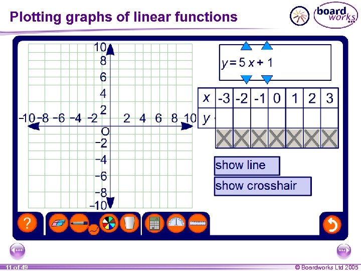 Plotting graphs of linear functions 11 of 49 © Boardworks Ltd 2005
 Contents A 8 Linear and real-life graphs A 8. 1 Linear graphs A 8. 2 Gradients and intercepts A 8. 3 Parallel and perpendicular lines A 8. 4 Interpreting real-life graphs A 8. 5 Distance-time graphs A 8. 6 Speed-time graphs 12 of 49 © Boardworks Ltd 2005
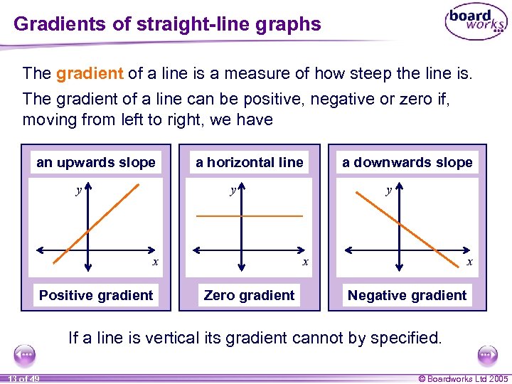 Gradients of straight-line graphs The gradient of a line is a measure of how steep the line is. The gradient of a line can be positive, negative or zero if, moving from left to right, we have an upwards slope y a horizontal line y y x x Positive gradient a downwards slope Zero gradient x Negative gradient If a line is vertical its gradient cannot by specified. 13 of 49 © Boardworks Ltd 2005
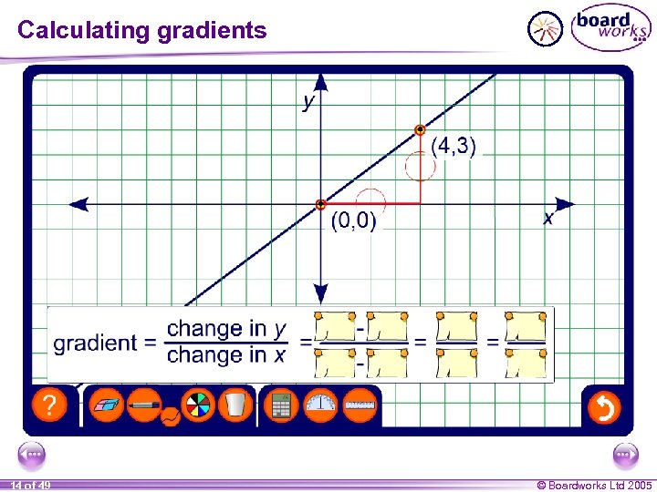 Calculating gradients 14 of 49 © Boardworks Ltd 2005
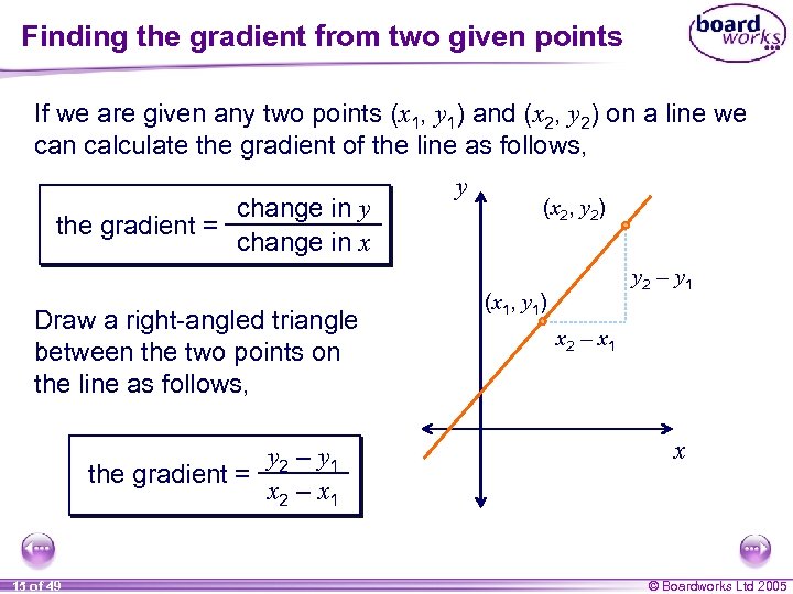 Finding the gradient from two given points If we are given any two points (x 1, y 1) and (x 2, y 2) on a line we can calculate the gradient of the line as follows, change in y the gradient = change in x Draw a right-angled triangle between the two points on the line as follows, y 2 – y 1 the gradient = x 2 – x 1 15 of 49 y (x 2, y 2) y 2 – y 1 (x 1, y 1) x 2 – x 1 x © Boardworks Ltd 2005
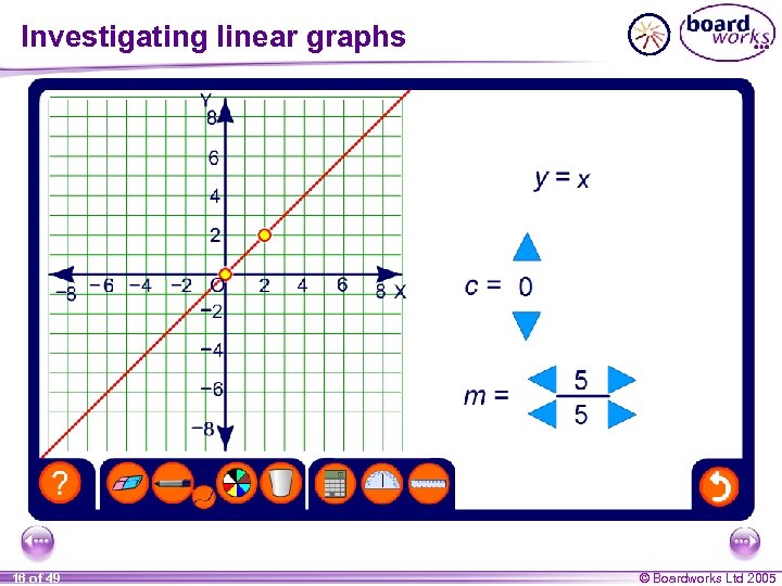 Investigating linear graphs 16 of 49 © Boardworks Ltd 2005
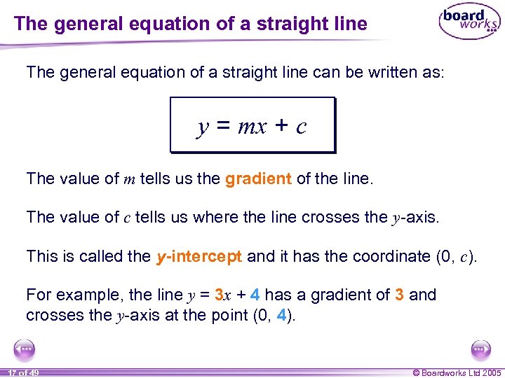 The general equation of a straight line can be written as: y = mx + c The value of m tells us the gradient of the line. The value of c tells us where the line crosses the y-axis. This is called the y-intercept and it has the coordinate (0, c). For example, the line y = 3 x + 4 has a gradient of 3 and crosses the y-axis at the point (0, 4). 17 of 49 © Boardworks Ltd 2005
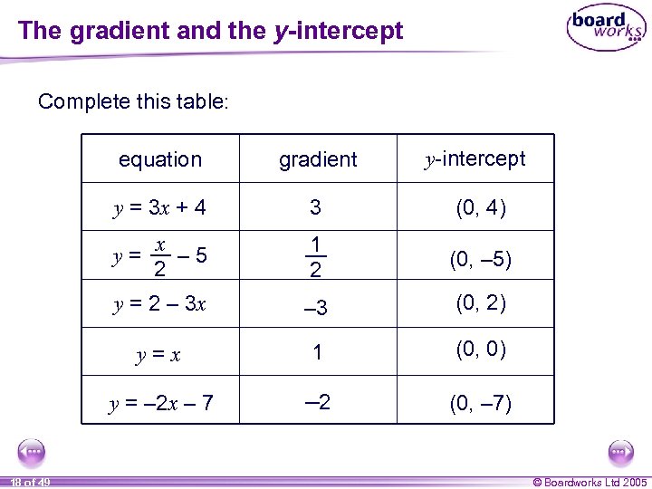 The gradient and the y-intercept Complete this table: equation gradient y-intercept y = 3 x + 4 3 (0, 4) x – 5 2 1 2 (0, – 5) y = 2 – 3 x – 3 (0, 2) y=x 1 (0, 0) y = – 2 x – 7 – 2 (0, – 7) y= 18 of 49 © Boardworks Ltd 2005
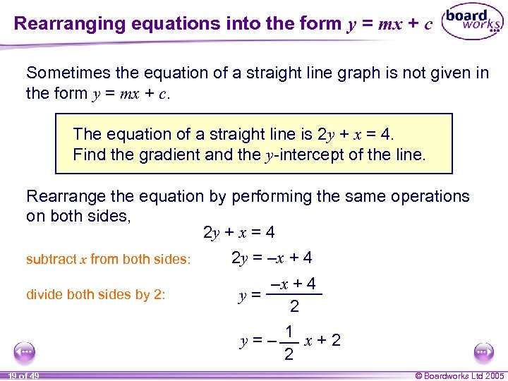 Rearranging equations into the form y = mx + c Sometimes the equation of a straight line graph is not given in the form y = mx + c. The equation of a straight line is 2 y + x = 4. Find the gradient and the y-intercept of the line. Rearrange the equation by performing the same operations on both sides, 2 y + x = 4 subtract x from both sides: divide both sides by 2: 2 y = –x + 4 y= 2 y=– 1 x+2 2 19 of 49 © Boardworks Ltd 2005
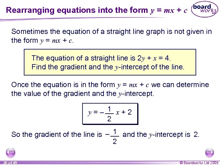 Rearranging equations into the form y = mx + c Sometimes the equation of a straight line graph is not given in the form y = mx + c. The equation of a straight line is 2 y + x = 4. Find the gradient and the y-intercept of the line. Once the equation is in the form y = mx + c we can determine the value of the gradient and the y-intercept. y=– 1 x+2 2 So the gradient of the line is – 1 and the y-intercept is 2. 2 20 of 49 © Boardworks Ltd 2005
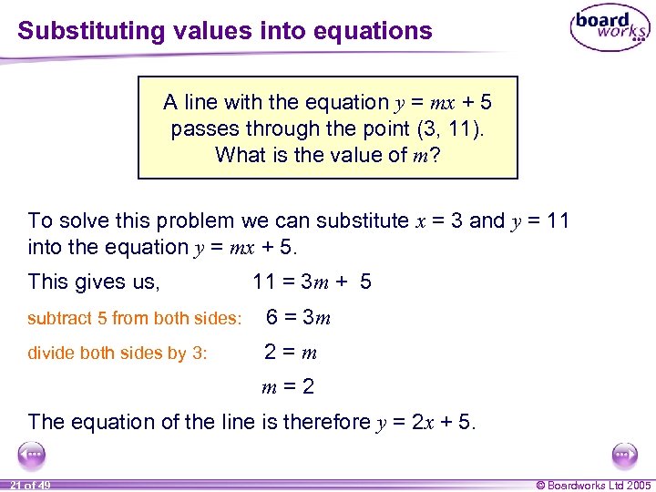 Substituting values into equations A line with the equation y = mx + 5 passes through the point (3, 11). What is the value of m? To solve this problem we can substitute x = 3 and y = 11 into the equation y = mx + 5. This gives us, 11 = 3 m + 5 subtract 5 from both sides: 6 = 3 m divide both sides by 3: 2=m m=2 The equation of the line is therefore y = 2 x + 5. 21 of 49 © Boardworks Ltd 2005
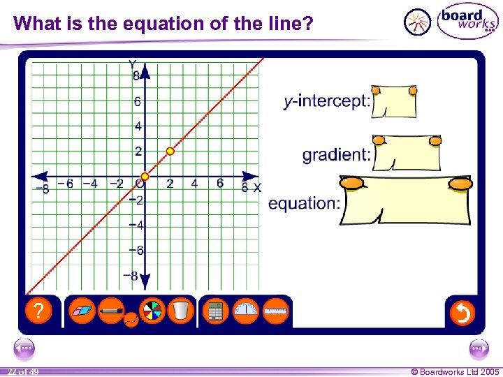 What is the equation of the line? 22 of 49 © Boardworks Ltd 2005
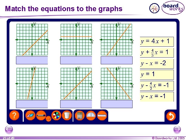 Match the equations to the graphs 23 of 49 © Boardworks Ltd 2005
 Contents A 8 Linear and real-life graphs A 8. 1 Linear graphs A 8. 2 Gradients and intercepts A 8. 3 Parallel and perpendicular lines A 8. 4 Interpreting real-life graphs A 8. 5 Distance-time graphs A 8. 6 Speed-time graphs 24 of 49 © Boardworks Ltd 2005
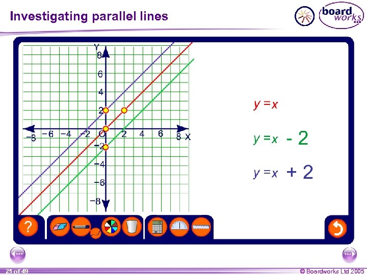 Investigating parallel lines 25 of 49 © Boardworks Ltd 2005
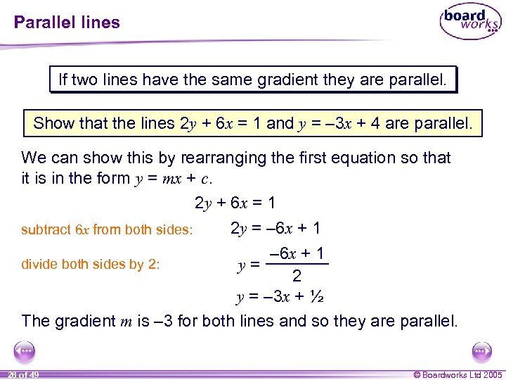 Parallel lines If two lines have the same gradient they are parallel. Show that the lines 2 y + 6 x = 1 and y = – 3 x + 4 are parallel. We can show this by rearranging the first equation so that it is in the form y = mx + c. 2 y + 6 x = 1 2 y = – 6 x + 1 subtract 6 x from both sides: – 6 x + 1 divide both sides by 2: y= 2 y = – 3 x + ½ The gradient m is – 3 for both lines and so they are parallel. 26 of 49 © Boardworks Ltd 2005
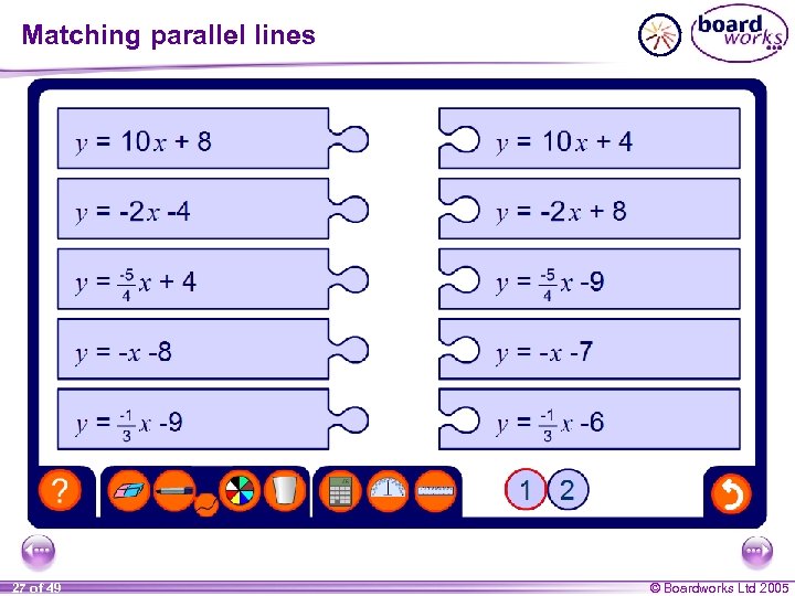 Matching parallel lines 27 of 49 © Boardworks Ltd 2005
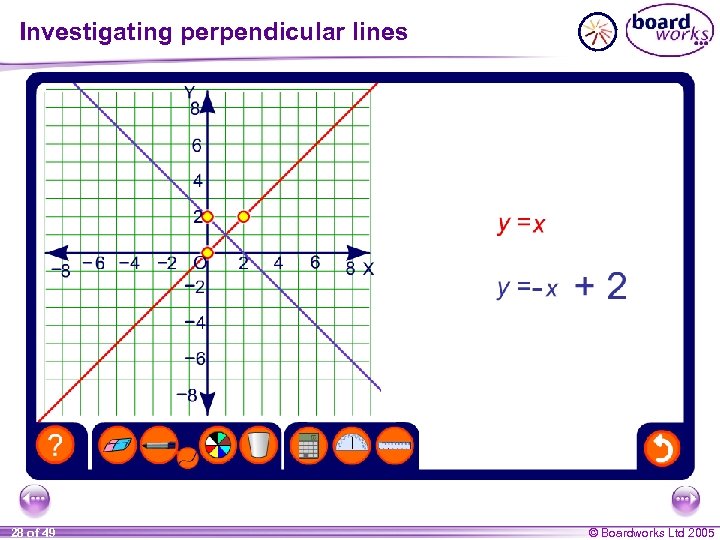 Investigating perpendicular lines 28 of 49 © Boardworks Ltd 2005
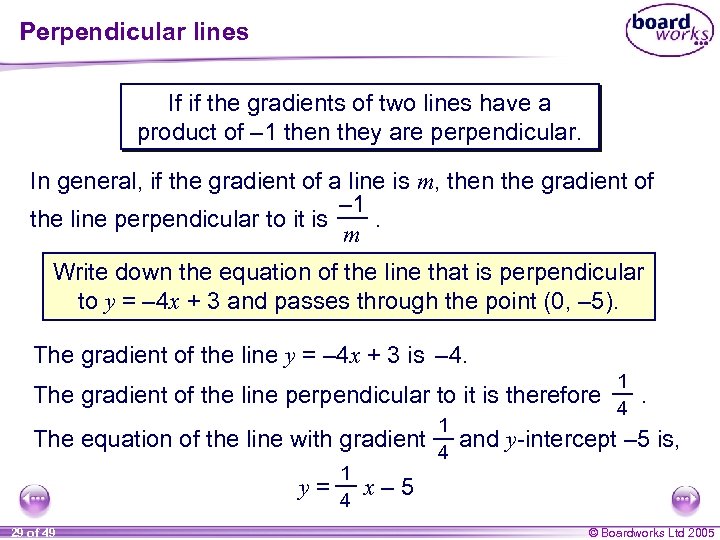 Perpendicular lines If if the gradients of two lines have a product of – 1 then they are perpendicular. In general, if the gradient of a line is m, then the gradient of – 1 the line perpendicular to it is. m Write down the equation of the line that is perpendicular to y = – 4 x + 3 and passes through the point (0, – 5). The gradient of the line y = – 4 x + 3 is – 4. 1 The gradient of the line perpendicular to it is therefore 4. 1 The equation of the line with gradient and y-intercept – 5 is, y= 29 of 49 1 4 4 x– 5 © Boardworks Ltd 2005
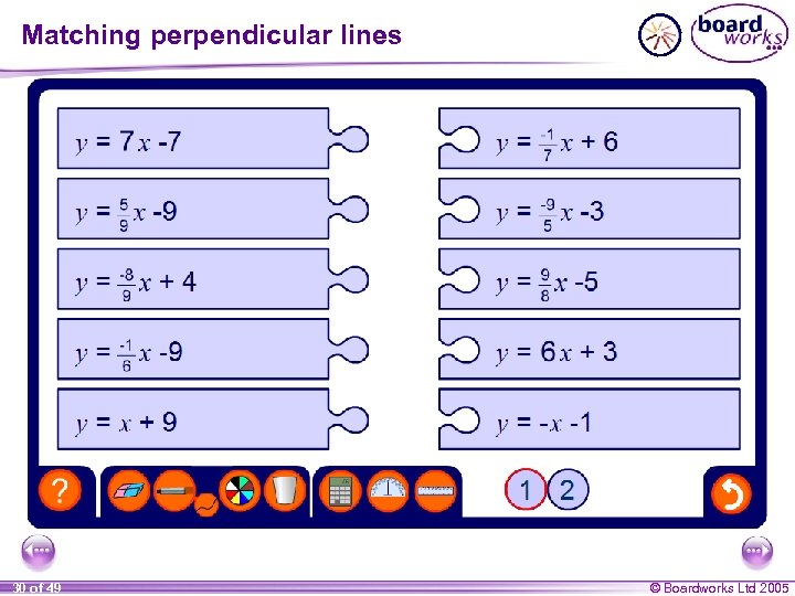 Matching perpendicular lines 30 of 49 © Boardworks Ltd 2005
 Contents A 8 Linear and real-life graphs A 8. 1 Linear graphs A 8. 2 Gradients and intercepts A 8. 3 Parallel and perpendicular lines A 8. 4 Interpreting real-life graphs A 8. 5 Distance-time graphs A 8. 6 Speed-time graphs 31 of 49 © Boardworks Ltd 2005
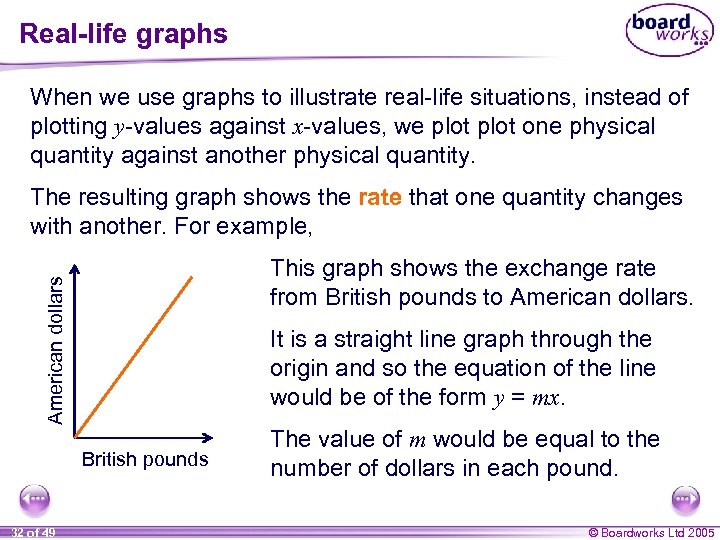 Real-life graphs When we use graphs to illustrate real-life situations, instead of plotting y-values against x-values, we plot one physical quantity against another physical quantity. The resulting graph shows the rate that one quantity changes with another. For example, American dollars This graph shows the exchange rate from British pounds to American dollars. It is a straight line graph through the origin and so the equation of the line would be of the form y = mx. British pounds 32 of 49 The value of thewould be m represent? What would m value of equal to the number of dollars in each pound. © Boardworks Ltd 2005
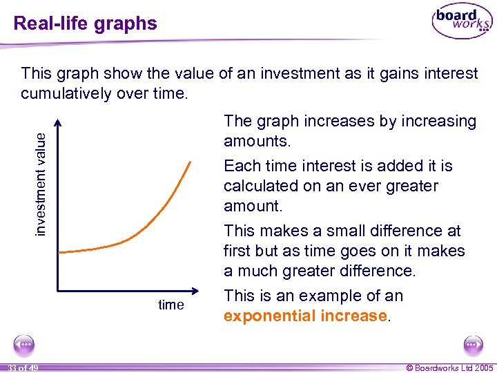 Real-life graphs This graph show the value of an investment as it gains interest cumulatively over time. investment value The graph increases by increasing amounts. Each time interest is added it is calculated on an ever greater amount. This makes a small difference at first but as time goes on it makes a much greater difference. time 33 of 49 This is an example of an exponential increase. © Boardworks Ltd 2005
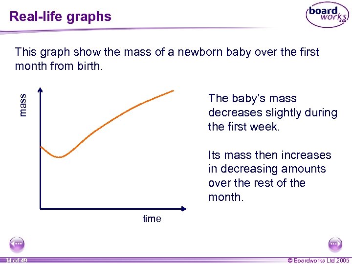 Real-life graphs This graph show the mass of a newborn baby over the first month from birth. mass The baby’s mass decreases slightly during the first week. Its mass then increases in decreasing amounts over the rest of the month. time 34 of 49 © Boardworks Ltd 2005
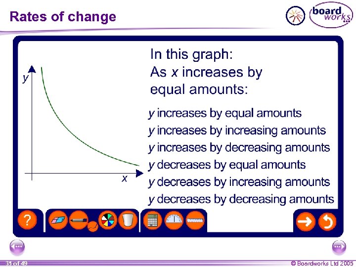 Rates of change 35 of 49 © Boardworks Ltd 2005
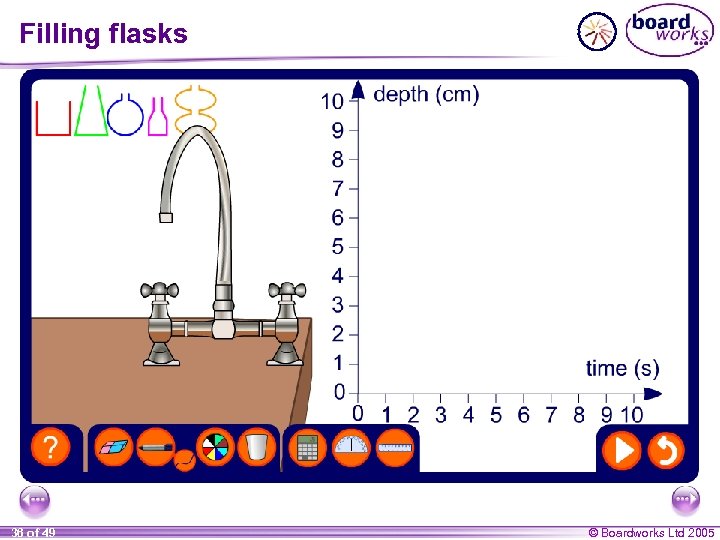 Filling flasks 36 of 49 © Boardworks Ltd 2005
 Contents A 8 Linear and real-life graphs A 8. 1 Linear graphs A 8. 2 Gradients and intercepts A 8. 3 Parallel and perpendicular lines A 8. 4 Interpreting real-life graphs A 8. 5 Distance-time graphs A 8. 6 Speed-time graphs 37 of 49 © Boardworks Ltd 2005
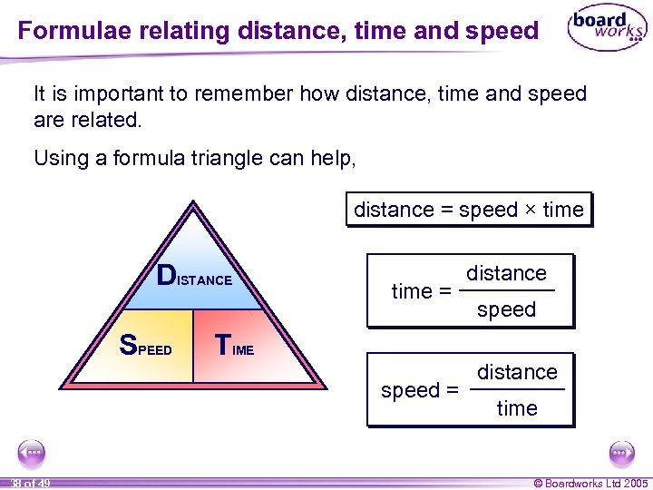 Formulae relating distance, time and speed It is important to remember how distance, time and speed are related. Using a formula triangle can help, distance = speed × time DISTANCE SPEED time = TIME speed = 38 of 49 distance speed distance time © Boardworks Ltd 2005
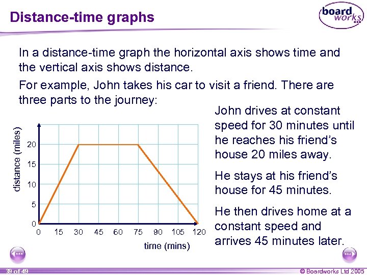 Distance-time graphs distance (miles) In a distance-time graph the horizontal axis shows time and the vertical axis shows distance. For example, John takes his car to visit a friend. There are three parts to the journey: John drives at constant speed for 30 minutes until he reaches his friend’s 20 house 20 miles away. 15 He stays at his friend’s house for 45 minutes. 10 5 0 0 15 30 45 60 75 90 105 120 time (mins) 39 of 49 He then drives home at a constant speed and arrives 45 minutes later. © Boardworks Ltd 2005
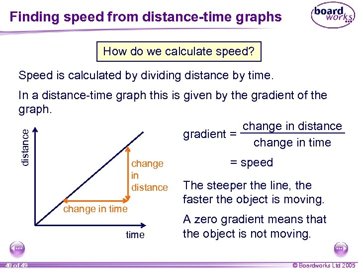 Finding speed from distance-time graphs How do we calculate speed? Speed is calculated by dividing distance by time. distance In a distance-time graph this is given by the gradient of the graph. change in distance gradient = change in time change in distance change in time 40 of 49 = speed The steeper the line, the faster the object is moving. A zero gradient means that the object is not moving. © Boardworks Ltd 2005
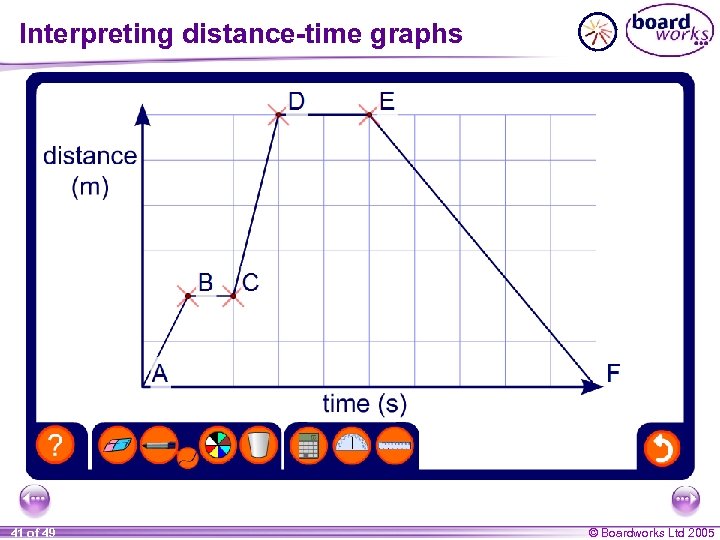 Interpreting distance-time graphs 41 of 49 © Boardworks Ltd 2005
 Distance-time graphs When a distance-time graph is linear the objects involved are moving at a constant speed. Most real-life objects do not always move at constant speed, however. It is more likely that they will speed up and slow down during the journey. Increase in speed over time is called acceleration = change in speed time It is measured in metres per second or m/s 2. When speed decreases over time is often is called deceleration. 42 of 49 © Boardworks Ltd 2005
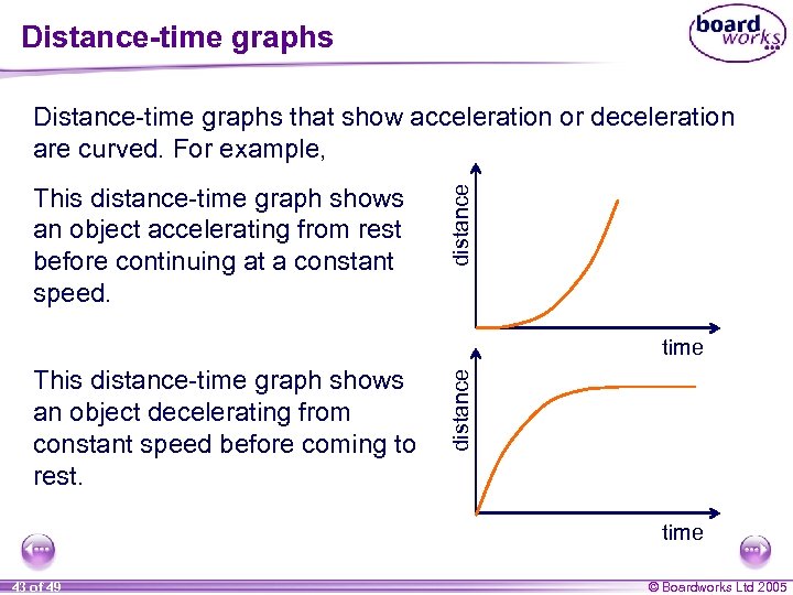 Distance-time graphs This distance-time graph shows an object accelerating from rest before continuing at a constant speed. distance Distance-time graphs that show acceleration or deceleration are curved. For example, This distance-time graph shows an object decelerating from constant speed before coming to rest. distance time 43 of 49 © Boardworks Ltd 2005
 Contents A 8 Linear and real-life graphs A 8. 1 Linear graphs A 8. 2 Gradients and intercepts A 8. 3 Parallel and perpendicular lines A 8. 4 Interpreting real-life graphs A 8. 5 Distance-time graphs A 8. 6 Speed-time graphs 44 of 49 © Boardworks Ltd 2005
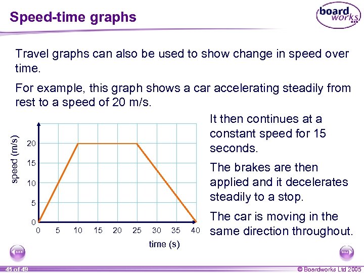 Speed-time graphs Travel graphs can also be used to show change in speed over time. speed (m/s) For example, this graph shows a car accelerating steadily from rest to a speed of 20 m/s. It then continues at a constant speed for 15 20 seconds. 15 The brakes are then applied and it decelerates steadily to a stop. 10 5 0 0 5 10 15 20 25 30 35 40 The car is moving in the same direction throughout. time (s) 45 of 49 © Boardworks Ltd 2005
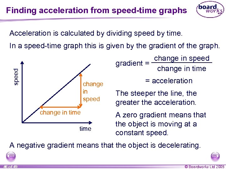 Finding acceleration from speed-time graphs Acceleration is calculated by dividing speed by time. In a speed-time graph this is given by the gradient of the graph. speed change in speed gradient = change in time change in speed change in time = acceleration The steeper the line, the greater the acceleration. A zero gradient means that the object is moving at a constant speed. A negative gradient means that the object is decelerating. 46 of 49 © Boardworks Ltd 2005
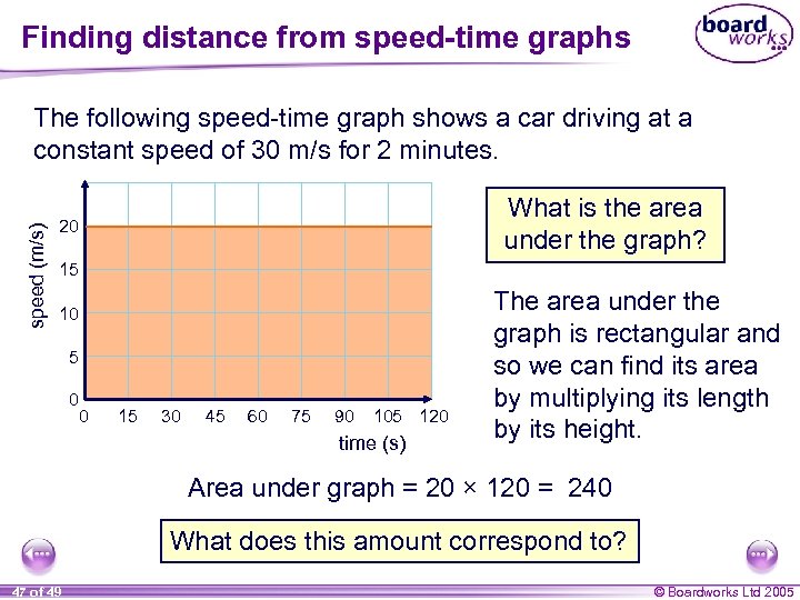 Finding distance from speed-time graphs speed (m/s) The following speed-time graph shows a car driving at a constant speed of 30 m/s for 2 minutes. What is the area under the graph? 20 15 10 5 0 0 15 30 45 60 75 90 105 120 time (s) The area under the graph is rectangular and so we can find its area by multiplying its length by its height. Area under graph = 20 × 120 = 240 What does this amount correspond to? 47 of 49 © Boardworks Ltd 2005
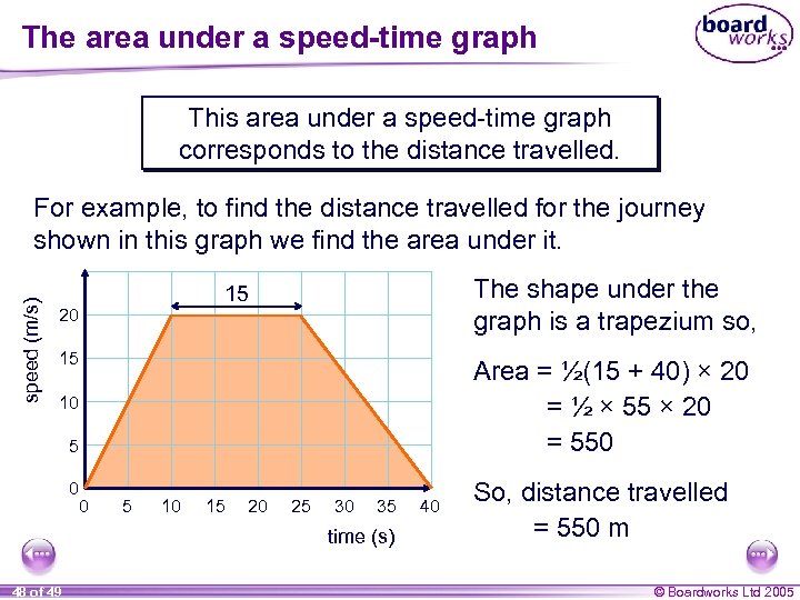 The area under a speed-time graph This area under a speed-time graph corresponds to the distance travelled. speed (m/s) For example, to find the distance travelled for the journey shown in this graph we find the area under it. The shape under the graph is a trapezium so, 15 20 15 Area = ½(15 + 40) × 20 = ½ × 55 × 20 = 550 10 5 0 0 5 10 15 20 25 30 35 time (s) 48 of 49 40 So, distance travelled = 550 m © Boardworks Ltd 2005
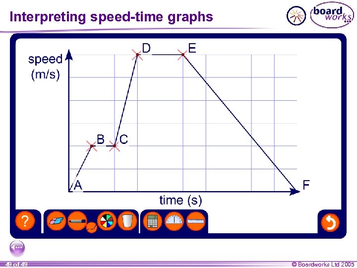 Interpreting speed-time graphs 49 of 49 © Boardworks Ltd 2005


