3 D ELECTRON DENSITY RECONSTRUCTION FROM THE SECCHI

3 D ELECTRON DENSITY RECONSTRUCTION FROM THE SECCHI CORONAGRAPHS and EUVI ONBOARD STEREO Jeffrey Newmark, John Cook Naval Research Laboratory (202) 767 -0244 newmark@nrl. navy. mil SECCHI SPD 2003. 1

Outline • SECCHI 3 D Reconstruction and Visualization Website: – http: //stereo. nrl. navy. mil/3 drv/3 dindex. html • Presentation Based on SECCHI Consortium Meeting, April 2004, CA • Overview of 3 D related activities by consortium • Details of selected activities • Heliospheric Imager – overview, science planning, CMEs • SMEI – not STEREO, early results, prelude for HI • Conclusions SECCHI SPD 2003. 2

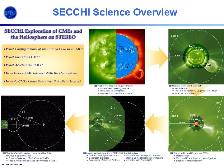SECCHI Science Overview SECCHI SPD 2003 <#>

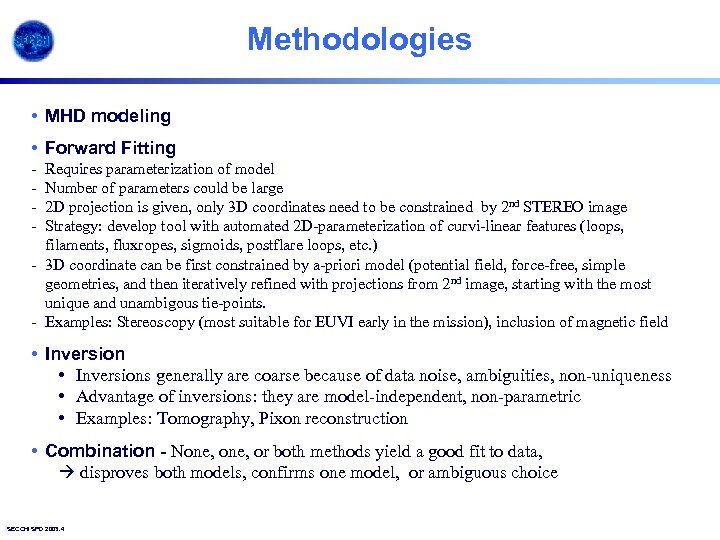Methodologies • MHD modeling • Forward Fitting - Requires parameterization of model Number of parameters could be large 2 D projection is given, only 3 D coordinates need to be constrained by 2 nd STEREO image Strategy: develop tool with automated 2 D-parameterization of curvi-linear features (loops, filaments, fluxropes, sigmoids, postflare loops, etc. ) - 3 D coordinate can be first constrained by a-priori model (potential field, force-free, simple geometries, and then iteratively refined with projections from 2 nd image, starting with the most unique and unambigous tie-points. - Examples: Stereoscopy (most suitable for EUVI early in the mission), inclusion of magnetic field • Inversions generally are coarse because of data noise, ambiguities, non-uniqueness • Advantage of inversions: they are model-independent, non-parametric • Examples: Tomography, Pixon reconstruction • Combination - None, or both methods yield a good fit to data, disproves both models, confirms one model, or ambiguous choice SECCHI SPD 2003. 4

SECCHI Group Activities (1) • NRL – 3 D Reconstruction of White Light Coronagraph Images from Multiple Viewpoints – Cook, Newmark, Reiser, Yahill – Tomography, Pixon reconstruction, 3 D data cube rendering – Differential Emission Measure (DEM) Tool for EUVI – Cook, Newmark – comparison with forward fitting models – Streamer Simulation – Vourlidas, Marque, Howard, Thernisien – model comparison to data, 3 D data cube rendering – CME Mass and Energetics Toolbox – Vourlidas, Thernisien, Howard – based on LASCO tools • JPL – Tie Point Tool – De Jong, Liewer, Hasll, Lorre – manual stereoscopy – Syn. LOS: synthetic LOS Tool for SECCHI white Light Images – Liewer, Hall, Lorre – 3 D data cube rendering • LMSAL/Rice – 3 D Reconstruction of Stereoscopic Images from EUVI – Aschwanden, Lemen, Wuelser, Alexander – forward modeling and constraint time series SECCHI SPD 2003. 5

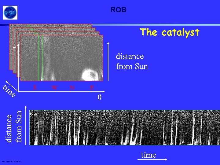
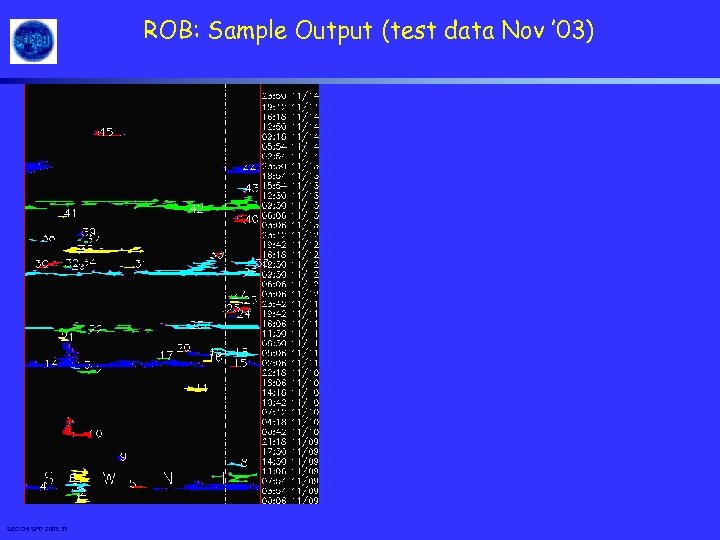
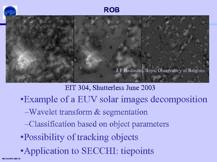
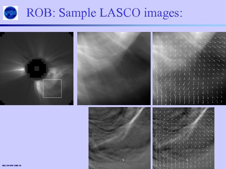
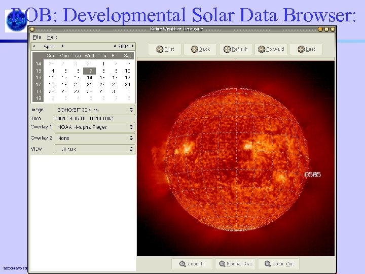
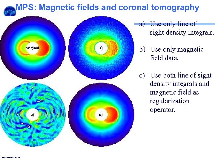
SECCHI Group Activities (2) • ROB – Computer Aided CME Tracking (CACTus) – Robbrecht, Berghmans, Lawrence, Van der Linden – pipeline processing automated CME catalog – based on LASCO – not reconstruction tool presently – Computer Aided EIT Wave and Dimming Detection – Podladchikova, Berghmans, Zhukov - pipeline processing automated EIT waves and dimming regions catalog – based on EIT – not reconstruction tool presently – Solar Weather Browser (SWB) – Nicula, Berghmans, Van der Linden – browse tool, not reconstruction tool presently – (Apparent) Velocity Map Construction – Hochedez, Gissot – full motion analysis software of EUV and WL using optical flow techniques – tracking, detection, stereoscopic reconstruction • MPS (formerly MPAe) – Finite Element Tomography Code (FETOC) – Inhester – 3 D tomography inversion code – coronal magnetic filed model can be used as a constraint – Stereoscopy of EUV loops – Portier-Fozzani (Athens), Inhester – parameterized, forward fitting loop model – Reconstruction of coronal magnetic fields (LINFF, NONLINFF) – Wiegelmann, Inhester – 3 D coronal magnetic field from boundary data, interfaces to provide reconstructed field for stereoscopy and tomography SECCHI SPD 2003. 6

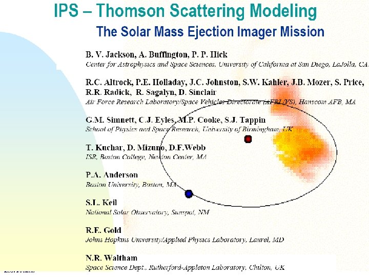
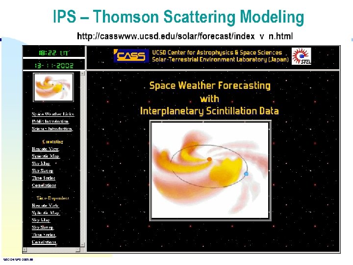
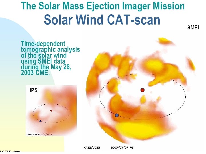
SECCHI Group Activities (3) • MPS/UB cont. – Real-time and 3 D visualization of STEREO images – Bothmer, Kraupe, Schwenn, Podlipnik, Cremades, Wiegelmann – planetarium display – 3 D Structure of CMEs: Origin, Internal Magnetic Field Configuration and Near-Sun Evolution – Bothmer, Cremades, Tripathi – comparison of model prediction (magnetic field + H-alpha based) and data • JHU/APL – Automatic solar feature recognition and classification – Rust, Bernasconi, La. Bonte – solar filaments, sigmoids, chirality, and CMEs – EUVI – helicity is important for 3 D modeling • Obs. de Paris – Combining Nancay Radio heliograph with SECCHI instruments – Pick, Kerdraon – identification of emitting coronal structures, source regions • SMEI (not SECCHI, but related to HI) - Jackson, Tappin, Hick, Webb – IPS and Thomson scattering Modeling/Tomography – solar wind model dependent, low resolution, developed from techniques based on Helios data SECCHI SPD 2003. 7

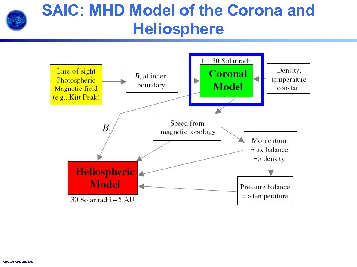
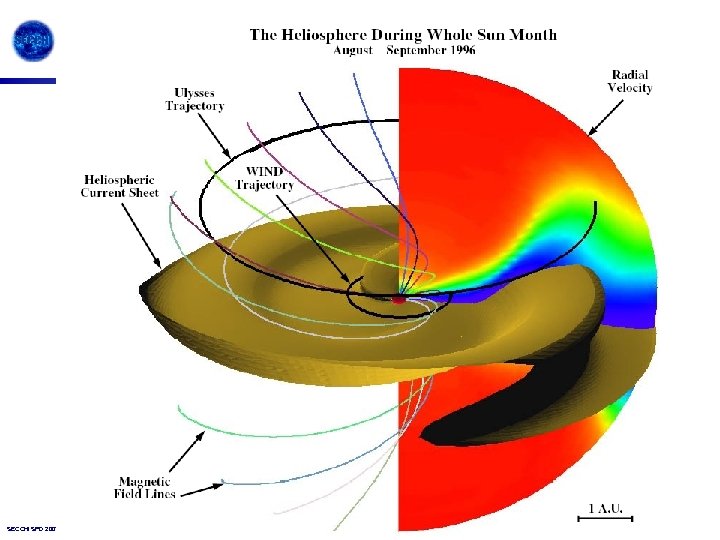
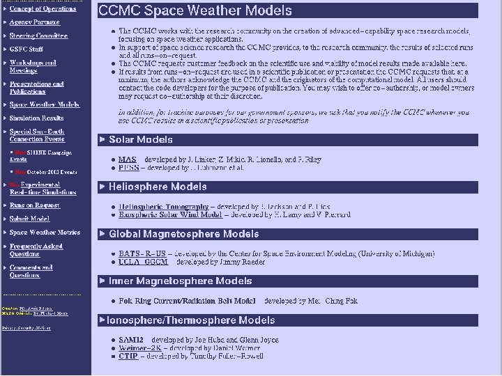
SECCHI Group Activities: MHD Modeling • NRL – Klimchuk, Antiochos, De. Vore, Karpen, Lopez-Fuentes, Lynch, Mac. Neice, Magara, Patsourakos – MHD CME initiation and propagation, Coronal loop structure, Coronal heating, Loop plasma evolution (incl. Prominences), Coronal hole evolution, Flux emergence, Active region structure – 3 D Visualization - Heliospace package, Developed with ARL (Tim Hall), Based on FAST (NASA/Ames) • SAIC – Mikic, Linker, Riley, Lionello – coronal and Heliospheric timde dependent MHD model = MAS • Univ. Alabama – Wu – MHD models • GSFC CCMC – hosts models SECCHI SPD 2003. 8

Specific Examples SECCHI SPD 2003. 9

NRL 3 D WL: Reconstruction • Strategy: Apply 3 D tomographic electron density reconstruction techniques to solar features from low corona through heliosphere to 1 AU. Utilize Brightness, polarized brightness, temporal, 2 D white light coronagraph images and synthetic models from 2/3 vantage points, construct (time dependent) 3 D electron density distribution. • Focus: Use theoretical CME models and existing LASCO observations prior to STEREO launch in order to predict the range of conditions and features where reconstruction techniques will be applicable. • Goal: Provide a practical tool that will achieve ~daily CME 3 D electron density models during the STEREO mission. • Study realistic complexities: Input Synthetic Models -> density structures (uniform vs. cavity vs. “realistic”), K/F corona, time dependence SECCHI SPD 2003. 10

NRL 3 D WL: Key Aspects • Renderer - Physics (Thomson scattering), tangential and radial polarization brightness, total brightness, finite viewer geometry, optically thin plasma. • Reconstruction Algorithm - PIXON (Pixon LLC), Pina, Puetter, Yahil (1993, 1995) - based upon minimum complexity, non-parametric, locally adaptive, iterative image reconstruction. Roughly analogous to multiscale (wavelet) methods (not as closely related to maximum entropy). – chosen for speed (large # voxels, up to 10^9): small number of iterations, intelligent guidance to declining complexity per iteration. Sample times have been 32 x 32 <15 minutes, 64 x 64 ~60 minutes, 128 x 128~6 hrs, (1 GHz PC). – Minimum complexity: With this underdetermined problem, we make minimal assumptions in order to progress. Another possibility is forward modelling, i. e. parameter fitting. Complementary approach. • Visualization - 3 D electron density distribution, time dependent (movies), multiple instrument, multiple spacecraft, physics MHD models. SECCHI SPD 2003. 11

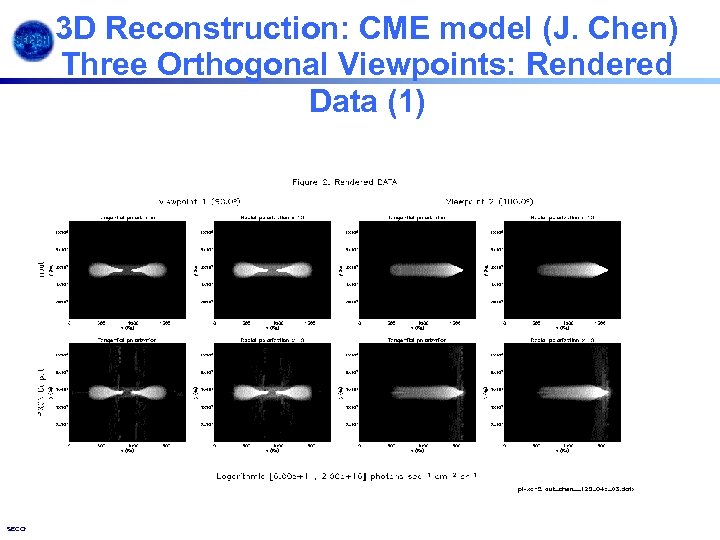3 D Reconstruction: CME model (J. Chen) Three Orthogonal Viewpoints: Rendered Data (1) SECCHI SPD 2003. 12

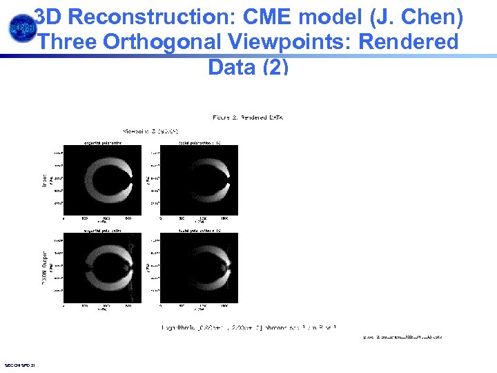3 D Reconstruction: CME model (J. Chen) Three Orthogonal Viewpoints: Rendered Data (2) SECCHI SPD 2003. 13

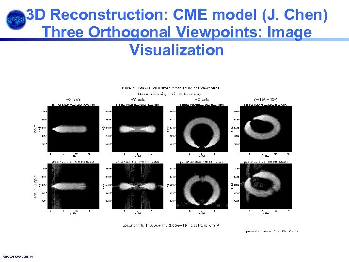3 D Reconstruction: CME model (J. Chen) Three Orthogonal Viewpoints: Image Visualization SECCHI SPD 2003. 14

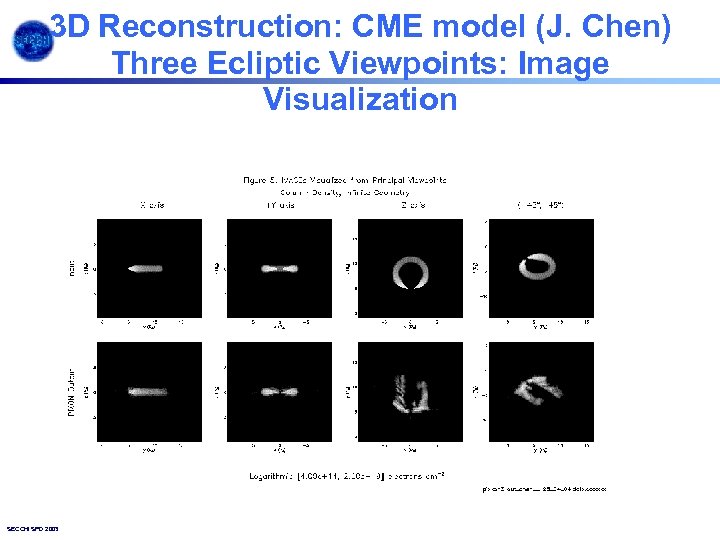3 D Reconstruction: CME model (J. Chen) Three Ecliptic Viewpoints: Image Visualization SECCHI SPD 2003. 15

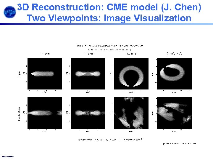3 D Reconstruction: CME model (J. Chen) Two Viewpoints: Image Visualization SECCHI SPD 2003. 16

NRL 2: Determining the Ne for a CME • For a transient event, such as a CME, the problem of determining K is quite straightforward, since we are only interested in the excess mass. • In this case we use a pre-event image to subtract the entire background from the image that contains the event. • Knowing the electron density, a simple conversion calculates the mass • Note: calculating the total excess mass only counts mass that comes up from below the occulting disk – it does not consider mass that has been transported from lower to higher heights, all within the field of view of that coronagraph • This procedure has been automated, and only needs to know the times of the event, the radial height of the leading edge, the central latitude or position angle and the angular span. Vourlidas et al 2003 has derived the following plot of the results of calculating the mass of over 4000 LASCO CMES SECCHI SPD 2003. 17

NRL 2: Determining Ne for a Coronal Structure • To calculate the electron density in a non-transient structure requires a different technique. • We have developed two different approaches, one using polarized brightness observations and the other using total brightness observations. The software for both of these approaches is available in the LASCO software tree. • In both techniques, a radial cut through the p. B or Bt corona, at a particular position angle, is obtained and then fit to a polynomial. Using an assumption of spherical symmetry, we then can then perform the inversion. • The p. B technique was developed by van de Hulst in the 1950 s and has been used for many years by many groups. It depends on the assumption that p. B = K, ie that all the other sources contributing to the observations are not polarized. This is usually not a bad assumption inside of about 3 -4 solar radii. • The Bt technique was developed by Hayes et al (2001). It depends on knowledge of each of the contributions given earlier. SECCHI SPD 2003. 18

NRL 2: Forward Modeling • Another technique we have started on is to assume a structure and then empirically generate a good fit to the observations. The difficultly with this approach is that the structure is only as good as your imagination and that many different structures may be equally suitable (or unsuitable) • This procedure allows you to specify the location in solar coordinates of a structure or combination of structures that are present in the corona and then allows you to view the resulting brightness image that would be generated from any angle. The structures must be expressed analytically. • We currently have various structures defined to represent possible streamer structures (slabs with a gaussian density, constant density cross section or gaussian-ellipsoid cross sections; a warped current sheet), a coronal hole. • We will be adding structures of possible CME representations – cone, spherical shell, ellipsoidal shell are currently envisioned. • We will also be making it more “user-friendly”. SECCHI SPD 2003. 19

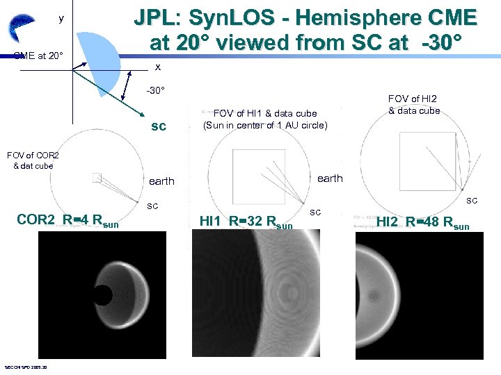y CME at 20° JPL: Syn. LOS - Hemisphere CME at 20° viewed from SC at -30° 20 -30 x -30° sc FOV of HI 1 & data cube (Sun in center of 1 AU circle) FOV of HI 2 & data cube FOV of COR 2 & dat cube earth sc COR 2 R=4 Rsun SECCHI SPD 2003. 20 HI 1 R=32 Rsun sc sc HI 2 R=48 Rsun

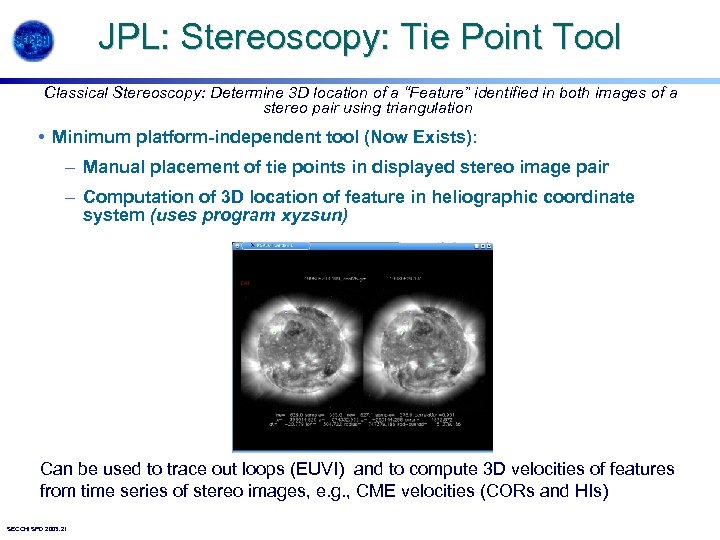JPL: Stereoscopy: Tie Point Tool Classical Stereoscopy: Determine 3 D location of a “Feature” identified in both images of a stereo pair using triangulation • Minimum platform-independent tool (Now Exists): – Manual placement of tie points in displayed stereo image pair – Computation of 3 D location of feature in heliographic coordinate system (uses program xyzsun) Can be used to trace out loops (EUVI) and to compute 3 D velocities of features from time series of stereo images, e. g. , CME velocities (CORs and HIs) SECCHI SPD 2003. 21

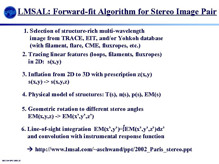LMSAL: Forward-fit Algorithm for Stereo Image Pair 1. Selection of structure-rich multi-wavelength image from TRACE, EIT, and/or Yohkoh database (with filament, flare, CME, fluxropes, etc. ) 2. Tracing linear features (loops, filaments, fluxropes) in 2 D: s(x, y) 3. Inflation from 2 D to 3 D with prescription z(x, y) s(x, y) -> s(x, y, z) 4. Physical model of structures: T(s), n(s), p(s), EM(s) 5. Geometric rotation to different stereo angles EM(x, y, z) -> EM(x’, y’, z’) 6. Line-of-sight integration EM(x’, y’)= EM(x’, y’, z’)dz’ and convolution with instrumental response function http: //www. lmsal. com/~aschwand/ppt/2002_Paris_stereo. ppt SECCHI SPD 2003. 22

LMSAL: 3 D Geometry [x(s), y(s), z(s)] of coronal structures, such as filaments, loops, arcades, flares, CMEs, … - Geometric definitions : 1 -dim parametrization along magnetic field lines is in low-beta plasma justified --> [x(s), y(s), z(s)] - Cross-sectionial variation for loops, --> A(s) - Start with tracing in 2 D in first STEREO image --> [x(s), y(s)] - Model for 3 D inflation z(s), e. g. semi-circular loops with vertical stretching factor z(s)=sqrt[(x(s)^2 + y(s)^2]*q_stretch - Forward-fitting to second STEREO image to determine q_stretch SECCHI SPD 2003. 23

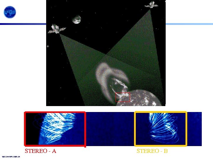STEREO - A SECCHI SPD 2003. 24 STEREO - B

LMSAL: Tracing linear features : --> [x(s), y(s)] High-pass filtering Feature tracing, reading coordinates, spline interpolation SECCHI SPD 2003. 25

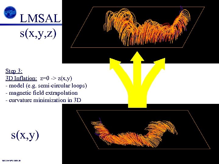LMSAL s(x, y, z) Step 3: 3 D Inflation: z=0 -> z(x, y) - model (e. g. semi-circular loops) - magnetic field extrapolation - curvature minimization in 3 D s(x, y) SECCHI SPD 2003. 26

* LMSAL: 3 D Fitting: F[x(s), y(s), z(s)] Volume rendering of coronal structures • Flux fitting in STEREO image • Volume filling of flux tube with sub-pixel sampling • Render cross-sections by superposition of loop fibers with subpixel • cross-sections: A=Sum(A_fiber), with w_fiber

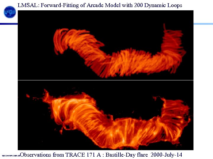LMSAL: Forward-Fitting of Arcade Model with 200 Dynamic Loops Observations from TRACE 171 A : Bastille-Day flare 2000 -July-14 SECCHI SPD 2003. 28

* LMSAL: 4 D Fitting: F[x(s), y(s), z(s), t] of coronal structures - Flux fitting in STEREO image #1 at time t 1 : - Flux fitting in STEREO image #2 at time t 1 - Sequential fitting of images #1, 2 at times t = t 2, t 3, …. , tn SECCHI SPD 2003. 29

LMSAL: 5 D Model: DEM [x(s), y(s), z(s), T(s), t] with dynamic physical model Ingredients for flare loop model : - 3 D Geometry [x(s), y(s), z(s)] - Dynamic evolution [x(s), y(s), z(s), t] - Heating function E_heat(s) - Thermal conduction - F_cond(s) - Radiative loss E_rad(s) = -n_e(s)^2 [T(s)] -> -> -> SECCHI SPD 2003. 30 Differential emission measure distribution d. EM(T, t)/d. T Line-of-sight integration EM(T)= n_e(z, T, t)^2 dz (STEREO angle) Instrumental response function R(T) Observed flux F(x, y, t)= EM(T, t) * R(T) d. T Flux fitting of 5 D-model onto 3 D flux F(x, y, t) for two stereo angles (4 D) and multiple temperature filters (5 D)

CACTus Computer Aided CME Tracking Eva Robbrecht David Berghmans Gareth Lawrence Royal Observatory of Belgium SECCHI SPD 2003. 31 ROB

ROB The catalyst r tim S W N E θ distance from Sun e distance from Sun time SECCHI SPD 2003. 32

ROB: Sample Output (test data Nov ’ 03) SECCHI SPD 2003. 33

ROB J-F Hochedez, Royal Observatory of Belgium EIT 304, Shutterless June 2003 • Example of a EUV solar images decomposition –Wavelet transform & segmentation –Classification based on object parameters • Possibility of tracking objects • Application to SECCHI: tiepoints SECCHI SPD 2003. 34

ROB: Sample LASCO images: SECCHI SPD 2003. 35

ROB: Developmental Solar Data Browser: SECCHI SPD 2003. 36

MPS: Magnetic fields tools Thomas Wiegelmann and Bernd Inhester STEREO/SECCHI has no magnetograph. Why do we develop magnetic field tools then? • Magnetic field dominates and structures the solar corona (magnetic pressure >> plasma pressure) • Coronal magnetic field is useful/necessary for Tomography and Stereoscopy. • Photospheric magnetic field data are (will be) available e. g. from Kitt Peak, SOHO/MDI (SOLIS, Solar-B) SECCHI SPD 2003. 37

MPS: Magnetic fields and coronal tomography a) Use only line of sight density integrals. b) Use only magnetic field data. c) Use both line of sight density integrals and magnetic field as regularization operator. SECCHI SPD 2003. 38

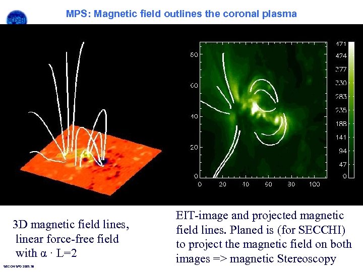MPS: Magnetic field outlines the coronal plasma 3 D magnetic field lines, linear force-free field with α · L=2 SECCHI SPD 2003. 39 EIT-image and projected magnetic field lines. Planed is (for SECCHI) to project the magnetic field on both images => magnetic Stereoscopy

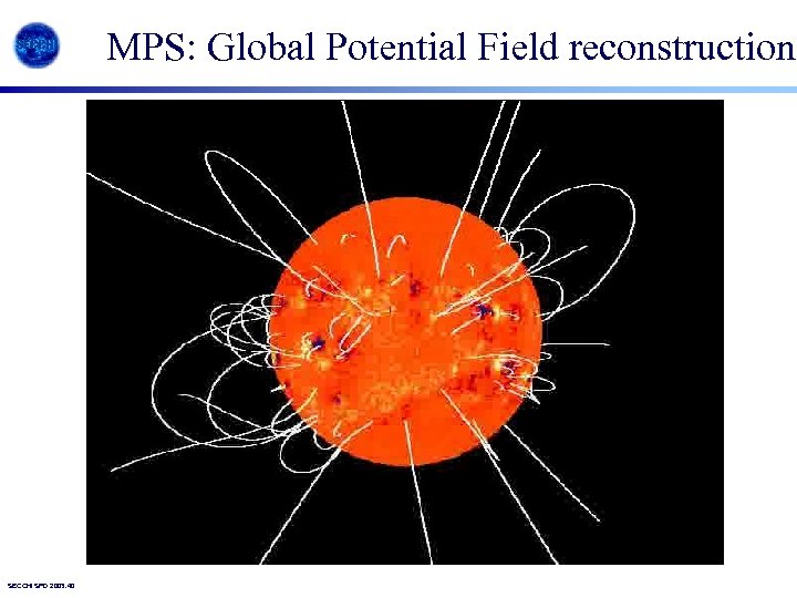MPS: Global Potential Field reconstruction SECCHI SPD 2003. 40

MPS: Summary magnetic fields • Potential magnetic fields and linear force free fields are popular due to their mathematic simplicity and available data. (e. g. from MDI on SOHO, Kitt Peak) • Nonlinear force free fields are necessary to describe active regions exactly. More challenging both observational and mathematical. • A consistent 3 D model of the solar corona requires tomographic inversion and magnetic reconstruction in one model. SECCHI SPD 2003. 41

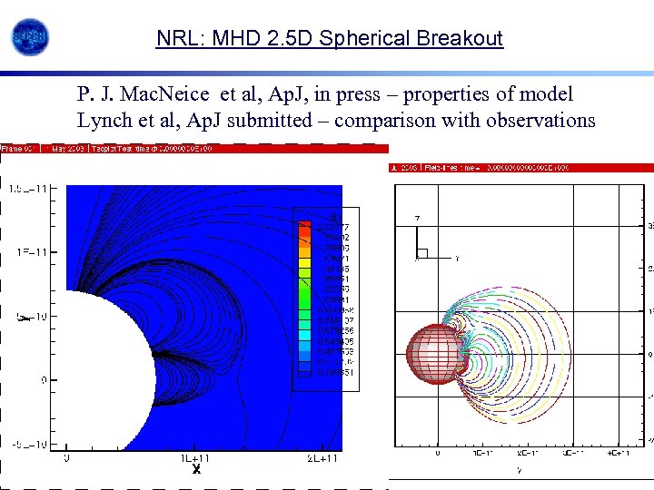NRL: MHD 2. 5 D Spherical Breakout P. J. Mac. Neice et al, Ap. J, in press – properties of model Lynch et al, Ap. J submitted – comparison with observations SECCHI SPD 2003. 42

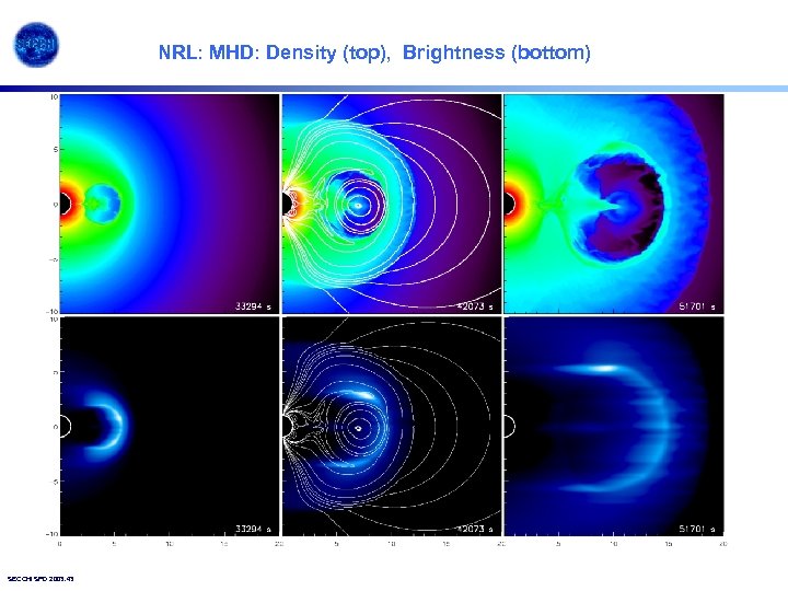NRL: MHD: Density (top), Brightness (bottom) SECCHI SPD 2003. 43

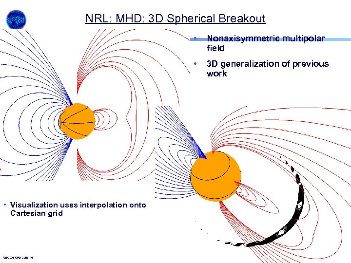NRL: MHD: 3 D Spherical Breakout • • • Visualization uses interpolation onto Cartesian grid SECCHI SPD 2003. 44 Nonaxisymmetric multipolar field 3 D generalization of previous work

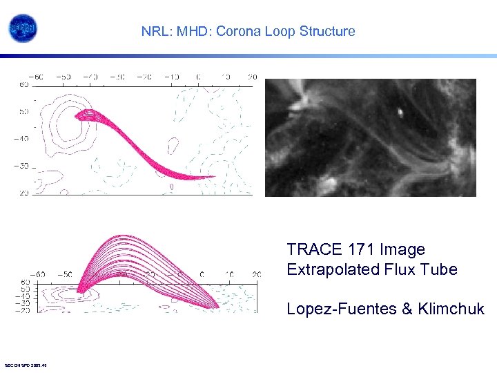NRL: MHD: Corona Loop Structure TRACE 171 Image Extrapolated Flux Tube Lopez-Fuentes & Klimchuk SECCHI SPD 2003. 45

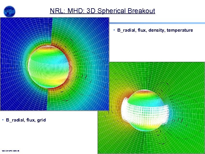NRL: MHD: 3 D Spherical Breakout • B_radial, flux, density, temperature • B_radial, flux, grid SECCHI SPD 2003. 46

SAIC: MAS Model Highlights SECCHI SPD 2003. 47

SAIC: MAS Model Highlights (cont. ) SECCHI SPD 2003. 48

SAIC: MHD Model of the Corona and Heliosphere SECCHI SPD 2003. 49

SECCHI SPD 2003. 50

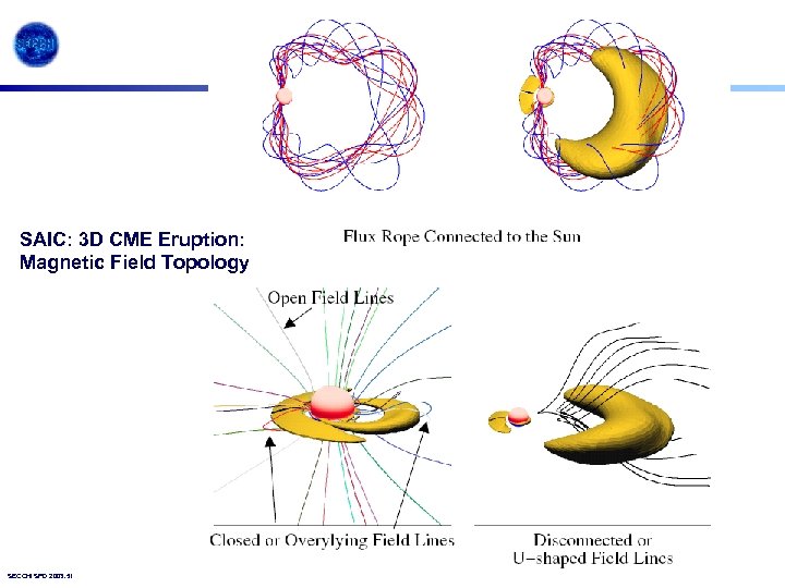SAIC: 3 D CME Eruption: Magnetic Field Topology SECCHI SPD 2003. 51

SECCHI SPD 2003. 52

SECCHI SPD 2003. 53

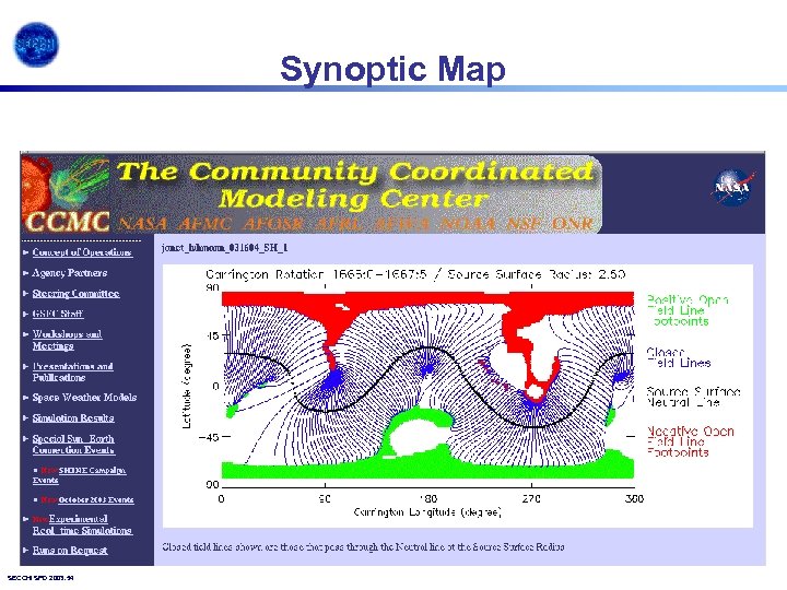Synoptic Map SECCHI SPD 2003. 54

Heliospheric Imager (HI) SECCHI SPD 2003. 55

Heliospheric Imager Ø HI Operations Document – R. Harrison Ø HI Image Simulation – C. Davis & R. Harrison Ø HI Operations Scenarios – R. Harrison & S. Matthews Ø HI Beacon Mode Specification – S. Matthews SECCHI SPD 2003. 56

Heliospheric Imager Ø HI in a nutshell: First opportunity to observe Earth-directed CMEs along the Sun-Earth line in interplanetary space - the first instrument to detect CMEs in a field of view including the Earth! First opportunity to obtain stereographic views of CMEs in interplanetary space - to investigate CME structure, evolution and propagation. Method: Occultation and baffle system, with wide angle view of the heliosphere, achieving light rejection levels of 3 x 10 -13 and 10 -14 of the solar brightness. SECCHI SPD 2003. 57

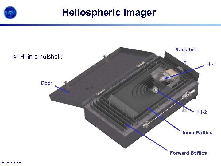Heliospheric Imager Radiator Ø HI in a nutshell: HI-1 Door HI-2 Inner Baffles Forward Baffles SECCHI SPD 2003. 58

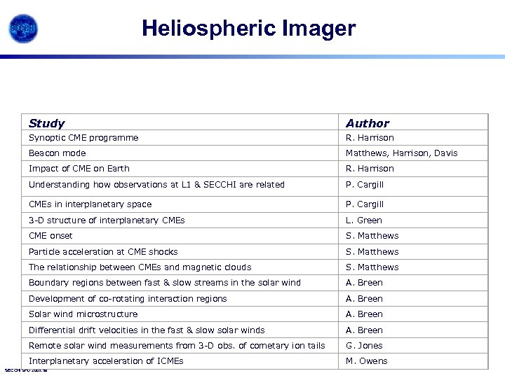Heliospheric Imager Study Author Synoptic CME programme R. Harrison Beacon mode Matthews, Harrison, Davis Impact of CME on Earth R. Harrison Understanding how observations at L 1 & SECCHI are related P. Cargill CMEs in interplanetary space P. Cargill 3 -D structure of interplanetary CMEs L. Green CME onset S. Matthews Particle acceleration at CME shocks S. Matthews The relationship between CMEs and magnetic clouds S. Matthews Boundary regions between fast & slow streams in the solar wind A. Breen Development of co-rotating interaction regions A. Breen Solar wind microstructure A. Breen Differential drift velocities in the fast & slow solar winds A. Breen Remote solar wind measurements from 3 -D obs. of cometary ion tails G. Jones Interplanetary acceleration of ICMEs M. Owens SECCHI SPD 2003. 59

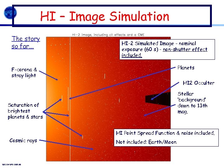HI – Image Simulation The story so far. . . HI-2 Simulated Image - nominal exposure (60 s) - non-shutter effect included. Planets F-corona & stray light HI 2 Occulter Stellar ‘background’ down to 13 th mag. Saturation of brightest planets & stars HI Point Spread Function & noise included. Cosmic rays SECCHI SPD 2003. 60 Not included: Earth/Moon

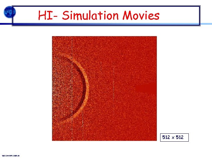HI- Simulation Movies 512 x 512 SECCHI SPD 2003. 61

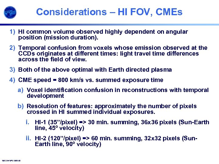Considerations – HI FOV, CMEs 1) HI common volume observed highly dependent on angular position (mission duration). 2) Temporal confusion from voxels whose emission observed at the CCDs originates at different times: light travel time differences across the field of view. 3) Both of the above optimal with Earth directed plasma 4) CME speed = 800 km/s vs. summed exposure time a) Voxel identification confusion in reconstructions with temporal development b) Resolution of features: approximately the number of pixels crossed in HI summed individual exposures. i. HI-1 (35”/pixel) => 30 min. summing, 36 x 36 pixels (Sun-Earth line, 45º velocity) ii. HI-2 (120”/pixel) => 60 min. summing, 32 x 32 pixels (Sun. Earth line, 90º velocity) SECCHI SPD 2003. 62

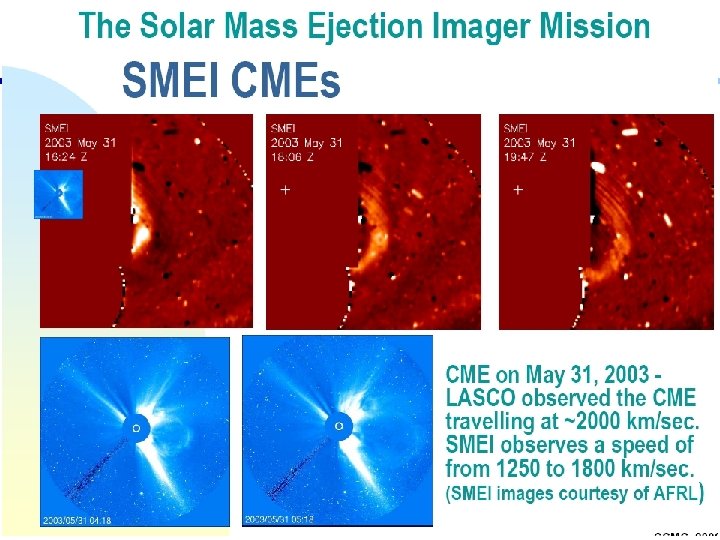
SMEI Early Results SECCHI SPD 2003. 63

SECCHI SPD 2003. 64

SECCHI SPD 2003. 65

SECCHI SPD 2003. 66

SECCHI SPD 2003. 67

Conclusions • Useful 3 D reconstructions are achievable! • There are real limitations that we must understand that will define which reconstructions are possible. • The reconstructions are significantly improved with the addition of a third viewpoint to the reconstruction, such as could be provided during the STEREO mission by an operating LASCO coronagraph on the SOHO spacecraft. • Application to SECCHI will require substantial effort and collaboration; we appreciate all help on scientific preparations. – Funding? • Web Site: http: //stereo. nrl. navy. mil/ (follow link to 3 D R&V). This contains past presentations and all necessary details to test reconstruction methods on sample problems. SECCHI SPD 2003. 68

BACKUP SLIDES SECCHI SPD 2003. 69

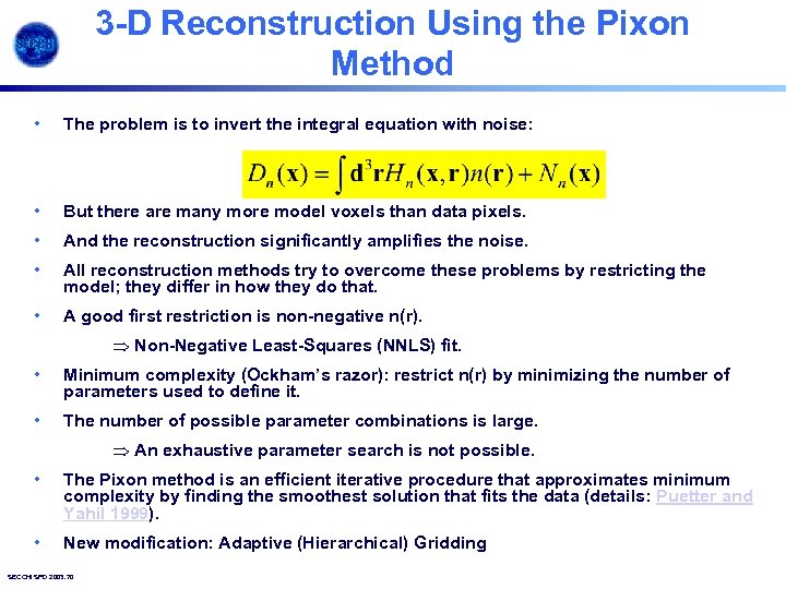3 -D Reconstruction Using the Pixon Method • The problem is to invert the integral equation with noise: • But there are many more model voxels than data pixels. • And the reconstruction significantly amplifies the noise. • All reconstruction methods try to overcome these problems by restricting the model; they differ in how they do that. • A good first restriction is non-negative n(r). Non-Negative Least-Squares (NNLS) fit. • Minimum complexity (Ockham’s razor): restrict n(r) by minimizing the number of parameters used to define it. • The number of possible parameter combinations is large. An exhaustive parameter search is not possible. • The Pixon method is an efficient iterative procedure that approximates minimum complexity by finding the smoothest solution that fits the data (details: Puetter and Yahil 1999). • New modification: Adaptive (Hierarchical) Gridding SECCHI SPD 2003. 70

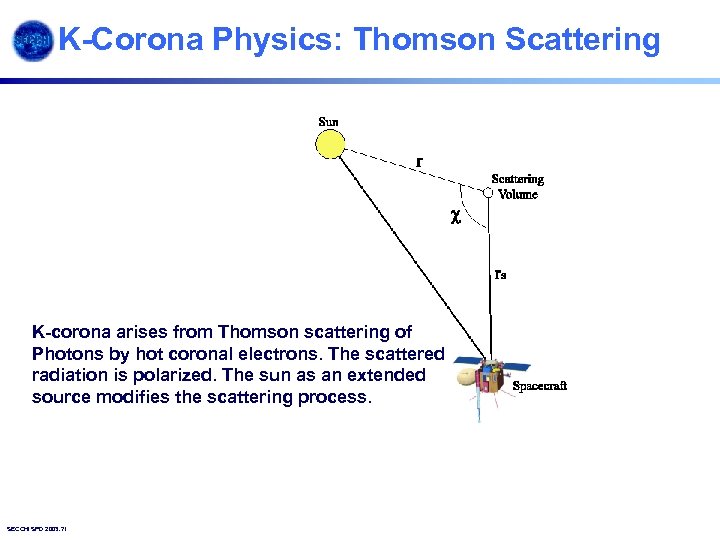K-Corona Physics: Thomson Scattering K-corona arises from Thomson scattering of Photons by hot coronal electrons. The scattered radiation is polarized. The sun as an extended source modifies the scattering process. SECCHI SPD 2003. 71

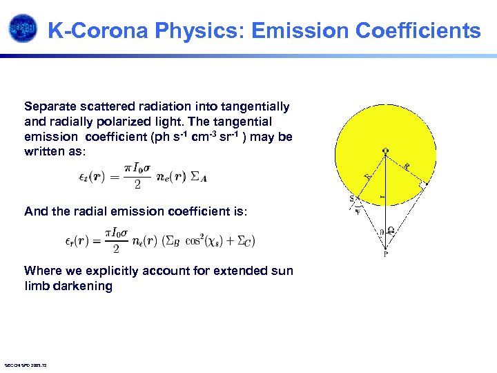K-Corona Physics: Emission Coefficients Separate scattered radiation into tangentially and radially polarized light. The tangential emission coefficient (ph s-1 cm-3 sr-1 ) may be written as: And the radial emission coefficient is: Where we explicitly account for extended sun limb darkening SECCHI SPD 2003. 72

PIXON: Adaptive (Hierarchical) Gridding • Naïve voxel size at the resolution of the projected detector pixels results in 109 voxels. • This is computationally unmanageable (or at least very time consuming). • The number of voxels greatly exceeds the number of independent data points, which is only 4 x 106. • We propose to solve both problems by using a hierarchical 3 -D grid, which is coarse where the (projected) data show n(r) to be smooth and is progressively refined where the data require n(r) to be more structured. • While the Pixon method does not require an adaptive grid, it can take advantage of it in imposing maximum smoothness to increase computational speed by a more efficient calculation. SECCHI SPD 2003. 73

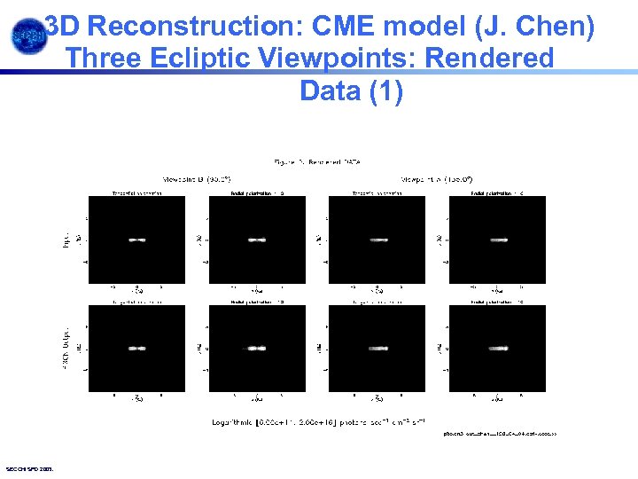3 D Reconstruction: CME model (J. Chen) Three Ecliptic Viewpoints: Rendered Data (1) SECCHI SPD 2003. 74

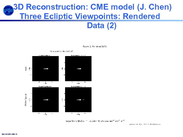3 D Reconstruction: CME model (J. Chen) Three Ecliptic Viewpoints: Rendered Data (2) SECCHI SPD 2003. 75

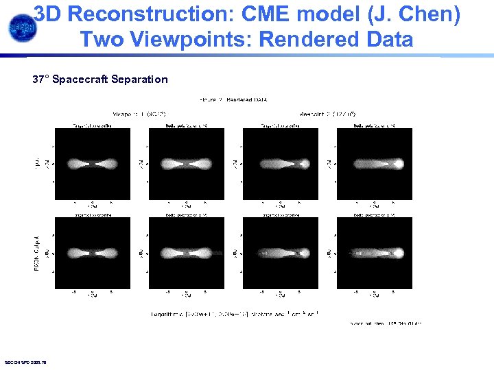3 D Reconstruction: CME model (J. Chen) Two Viewpoints: Rendered Data 37° Spacecraft Separation SECCHI SPD 2003. 76