2014 Examples of Traffic Video •

2014 Examples of Traffic

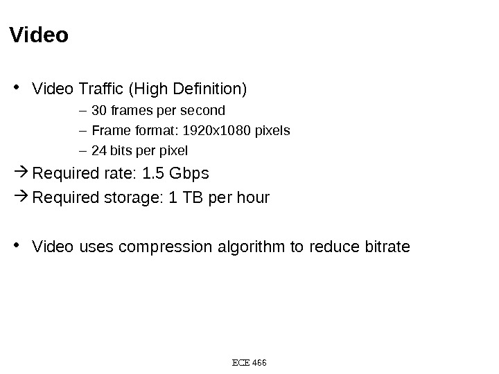
Video • Video Traffic (High Definition) – 30 frames per second – Frame format: 1920 x 1080 pixels – 24 bits per pixel Required rate: 1. 5 Gbps Required storage: 1 TB per hour • Video uses compression algorithm to reduce bitrate

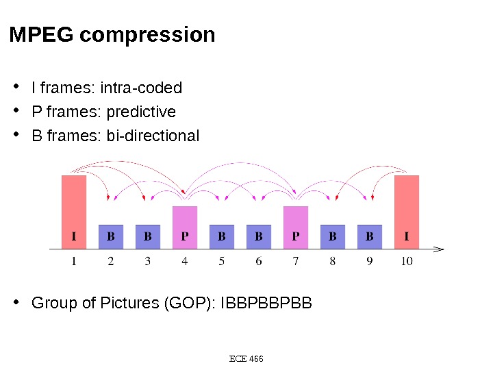
MPEG compression • I frames: intra-coded • P frames: predictive • B frames: bi-directional • Group of Pictures (GOP): IBBPBBP

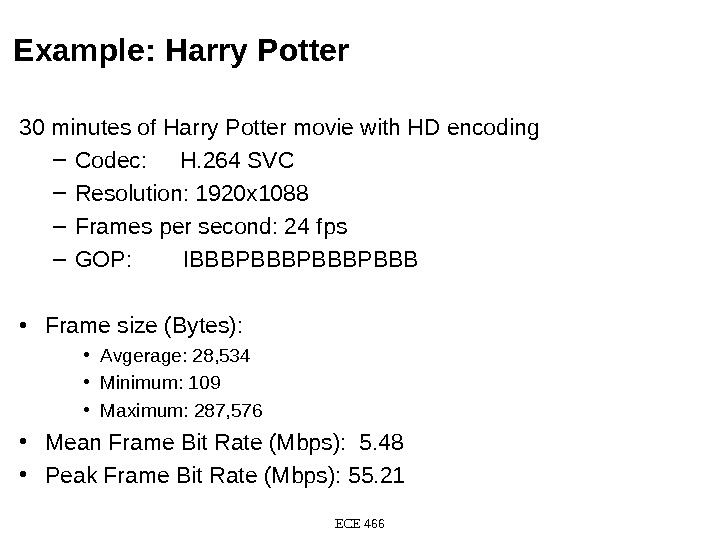
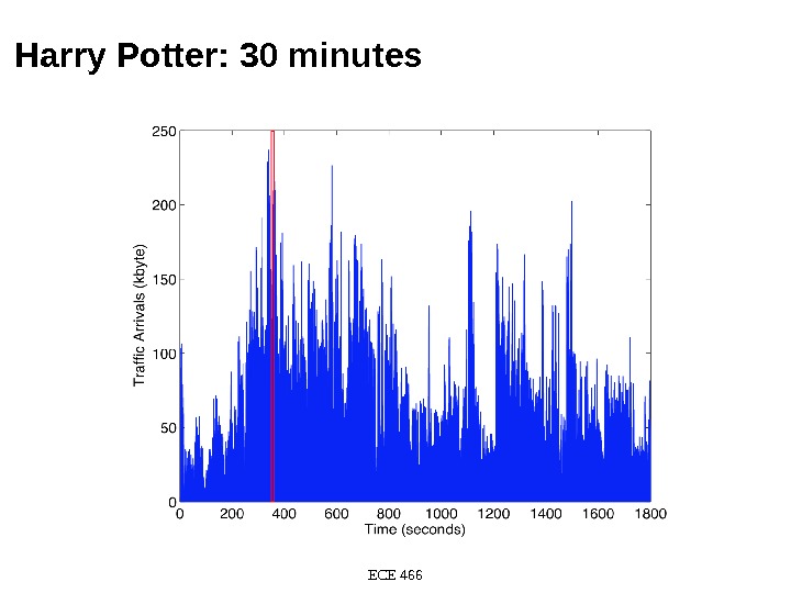
Example: Harry Potter 30 minutes of Harry Potter movie with HD encoding – Codec: H. 264 SVC – Resolution: 1920 x 1088 – Frames per second: 24 fps – GOP: IBBBPBBBPBBB • Frame size (Bytes): • Avgerage: 28, 534 • Minimum: 109 • Maximum: 287, 576 • Mean Frame Bit Rate (Mbps): 5. 48 • Peak Frame Bit Rate (Mbps): 55.

Harry Potter: 30 minutes

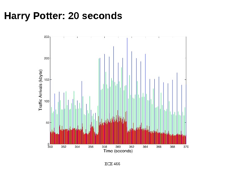
Harry Potter: 20 seconds

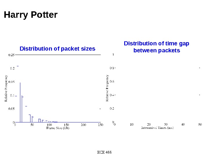
Harry Potter ECE 466 Distribution of packet sizes Distribution of time gap between packets

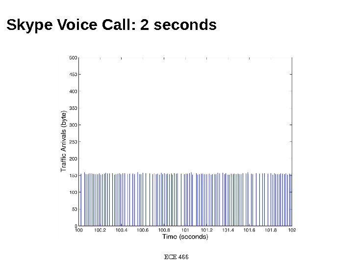
Voice • Standard (Pulse Code Modulation) voice encoding: – 8000 samples per second (8 k. Hz) – 8 bits per sample Bit rate: 64 kbps • Better quality with higher sampling rate and larger samples • CD encoding: – 44 k. Hz sampling rate – 16 bits per sample – 2 channels Bit rate: 1. 4 Mbps • Packet voice collects multiple samples in once packet • Modern voice encoding schemes also use compression and silent suppression

Skype Voice Call: 6 minutes ECE 466 • SVOPC encoding, one direction of 2 -way call Dark blue: UDP traffic Light blue: TCP traffic

Skype Voice Call: 2 seconds

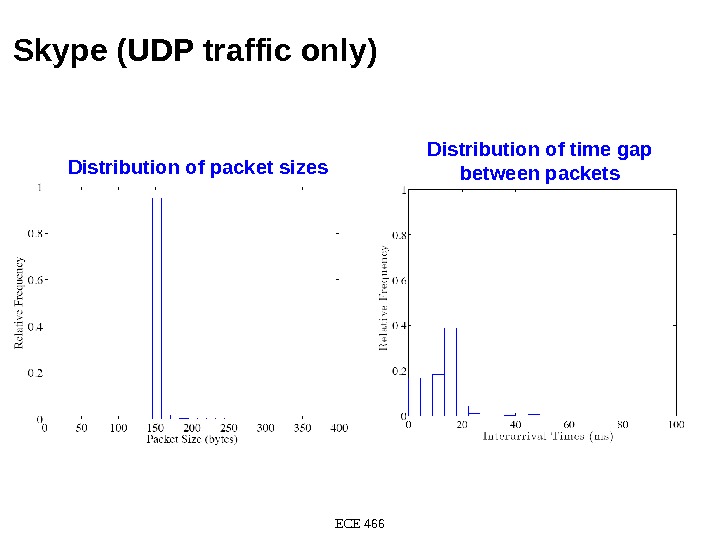
Skype (UDP traffic only) ECE 466 Distribution of packet sizes Distribution of time gap between packets

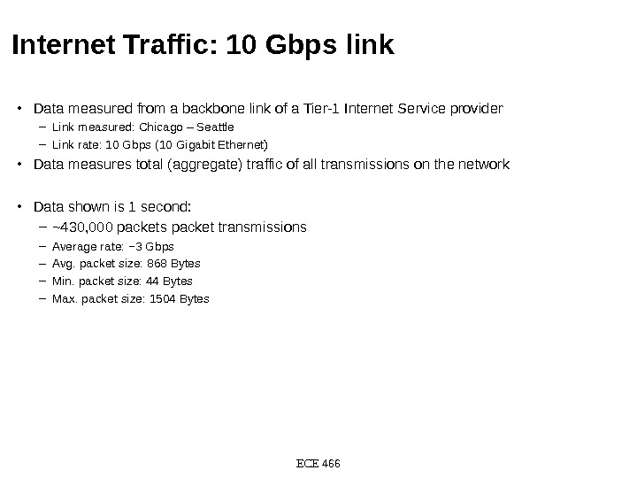
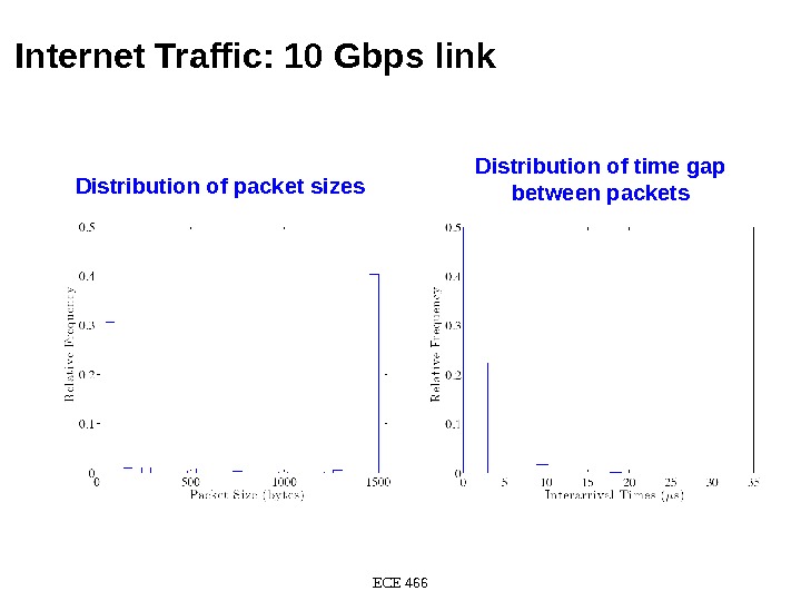
Internet Traffic: 10 Gbps link • Data measured from a backbone link of a Tier-1 Internet Service provider – Link measured: Chicago – Seattle – Link rate: 10 Gbps (10 Gigabit Ethernet) • Data measures total (aggregate) traffic of all transmissions on the network • Data shown is 1 second: – ~430, 000 packets packet transmissions – Average rate: ~3 Gbps – Avg. packet size: 868 Bytes – Min. packet size: 44 Bytes – Max. packet size: 1504 Bytes

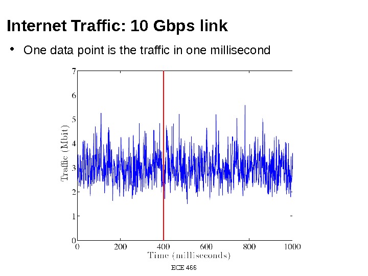
Internet Traffic: 10 Gbps link ECE 466 • One data point is the traffic in one millisecond

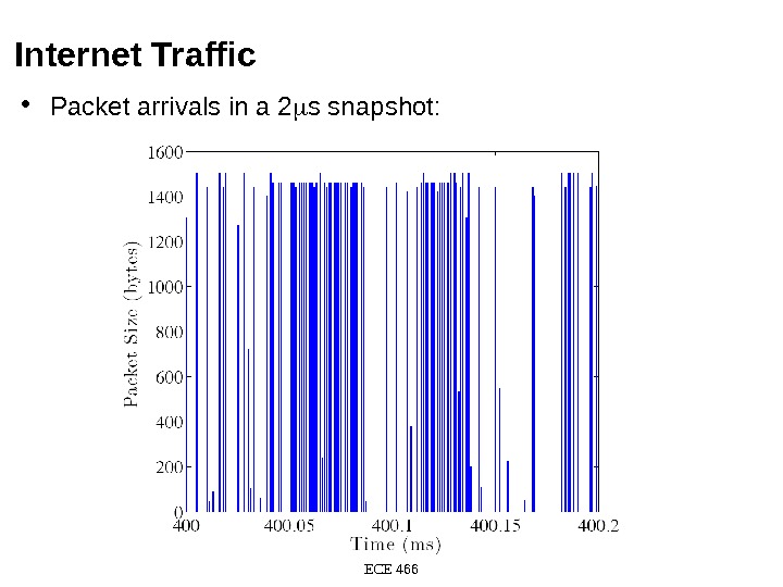
Internet Traffic ECE 466 • Packet arrivals in a 2 s snapshot:

Internet Traffic: 10 Gbps link ECE 466 Distribution of packet sizes Distribution of time gap between packets

Data Traffic: “Bellcore Traces” • Data measured on an Ethernet network at Bellcore Labs with 10 Mbps • Data measures total (aggregate) traffic of all transmissions on the network • Measurements from 1989 • One of the first systematic analyses of network measurements

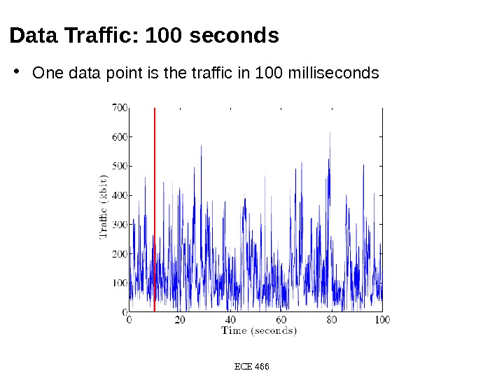
Data Traffic: 100 seconds ECE 466 • One data point is the traffic in 100 milliseconds

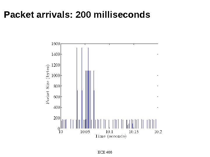
Packet arrivals: 200 milliseconds

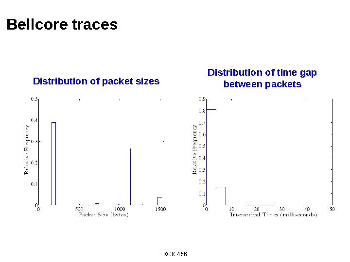
Bellcore traces ECE 466 Distribution of packet sizes Distribution of time gap between packets

Some background on Lab

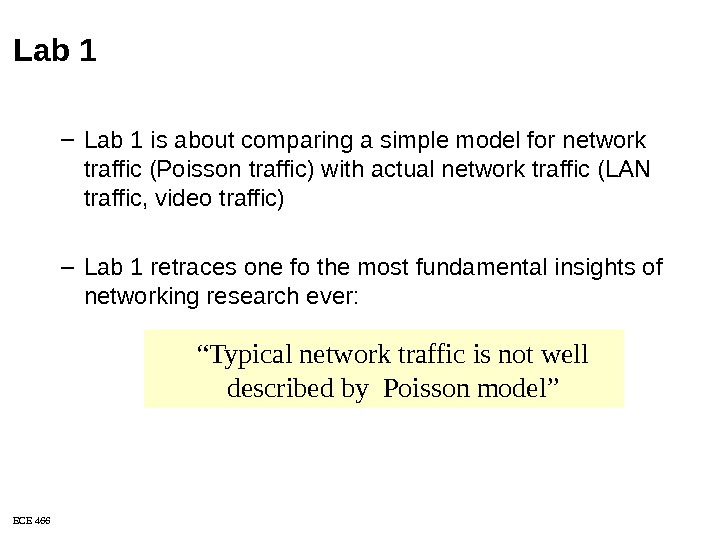
ECE 466 “ Typical network traffic is not well described by Poisson model”Lab 1 – Lab 1 is about comparing a simple model for network traffic (Poisson traffic) with actual network traffic (LAN traffic, video traffic) – Lab 1 retraces one fo the most fundamental insights of networking research ever:

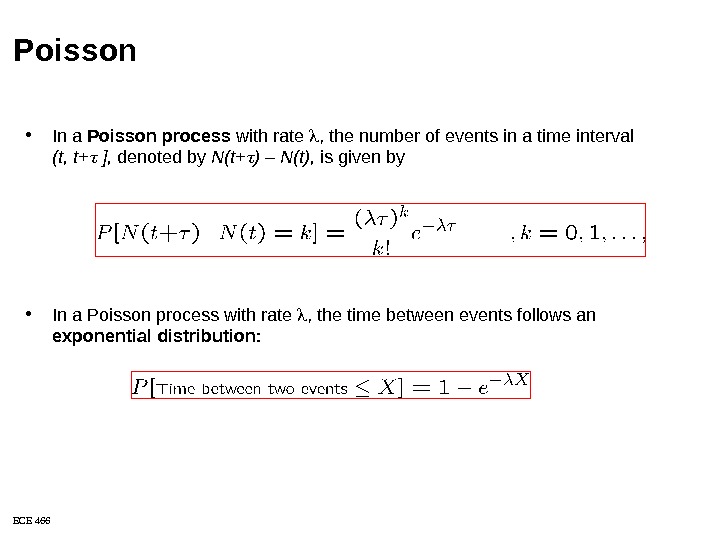
ECE 466 Poisson • In a Poisson process with rate , the number of events in a time interval (t, t+ ], denoted by N(t+ ) – N(t), is given by • In a Poisson process with rate , the time between events follows an exponential distribution:

ECE 466 In the Past… • Before there were packet networks there was the circuit-switched telephone network • Traffic modeling of telephone networks was the basis for initial network models – Assumed Poisson arrival process of new calls – Assumed Poisson call duration Source: Prof. P. Barford (edited)

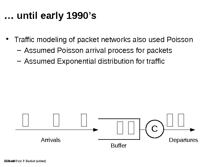
ECE 466… until early 1990 ’s • Traffic modeling of packet networks also used Poisson – Assumed Poisson arrival process for packets – Assumed Exponential distribution for traffic Source: Prof. P. Barford (edited)C Arrivals. Departures Buffer

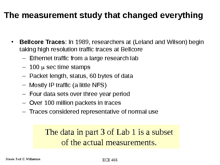
ECE 466 The measurement study that changed everything • Bellcore Traces : In 1989, researchers at (Leland Wilson) begin taking high resolution traffic traces at Bellcore – Ethernet traffic from a large research lab – 100 sec time stamps – Packet length, status, 60 bytes of data – Mostly IP traffic (a little NFS) – Four data sets over three year period – Over 100 million packets in traces – Traces considered representative of normal use Source: Prof. C. Williamson The data in part 3 of Lab 1 is a subset of the actual measurements.

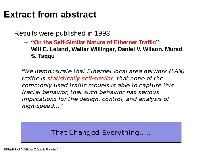
ECE 466 That Changed Everything…. . Extract from abstract Results were published in 1993 – “ On the Self-Similar Nature of Ethernet Traffic ” Will E. Leland, Walter Willinger, Daniel V. Wilson, Murad S. Taqqu “ We demonstrate that Ethernet local area network (LAN) traffic is statistically self-similar , that none of the commonly used traffic models is able to capture this fractal behavior, that such behavior has serious implications for the design, control, and analysis of high-speed…” Source: Prof. V. Mishra, Columbia U. (edited)

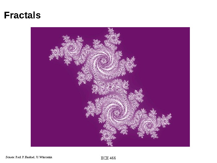
ECE 466 Fractals Source: Prof. P. Barford, U. Wisconsin

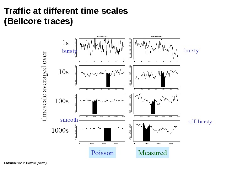
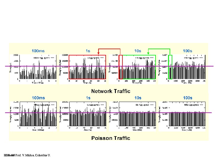
ECE 466 Traffic at different time scales (Bellcore traces) bursty still bursty Source: Prof. P. Barford (edited)

ECE 466 Source: Prof. V. Mishra, Columbia U.

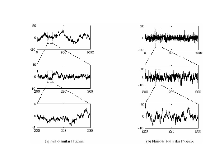
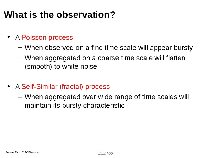
ECE 466 What is the observation? • A Poisson process – When observed on a fine time scale will appear bursty – When aggregated on a coarse time scale will flatten (smooth) to white noise • A Self-Similar (fractal) process – When aggregated over wide range of time scales will maintain its bursty characteristic Source: Prof. C. Williamson

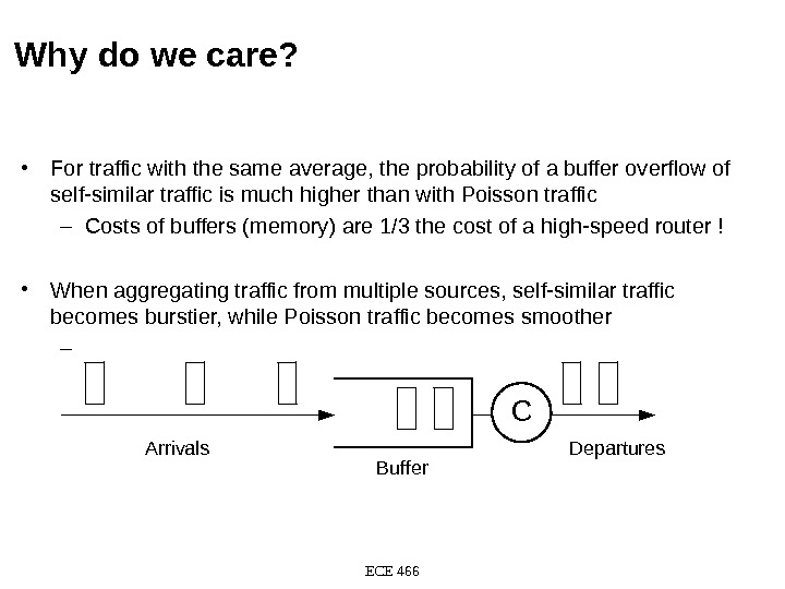
ECE 466 Why do we care? • For traffic with the same average, the probability of a buffer overflow of self-similar traffic is much higher than with Poisson traffic – Costs of buffers (memory) are 1/3 the cost of a high-speed router ! • When aggregating traffic from multiple sources, self-similar traffic becomes burstier, while Poisson traffic becomes smoother – C Arrivals. Departures Buffer

ECE 466 • The objective in Lab 1 is to observe self-similarity and obtain a sense. • The challenge of Lab 1: – The Bellcore trace for Part 4 contains 1, 000 packets – The computers in the lab are not happy with that many packets – Reducing the number of packets in plots, may reduce opportunities to discover self-similarity effect. Self-similarity