14 Execution strategies 14 1 Introduction Opportunistic algorithms

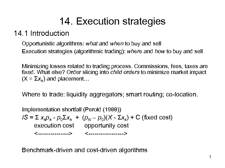14. Execution strategies 14. 1 Introduction Opportunistic algorithms: what and when to buy and sell Execution strategies (algorithmic trading): where and how to buy and sell Minimizing losses related to trading process. Commissions, fees, taxes are fixed. What else? Order slicing into child orders to minimize market impact (X = Σxk) and placement… Where to trade: liquidity aggregators; smart routing; co-location. Implementation shortfall (Perold (1988)) IS = Σ xkpk - p 0Σxk + (p. N – p 0)(X - Σxk) + C (fixed cost) execution cost opportunity cost <--------> <---------> Benchmark-driven and cost-driven algorithms 1

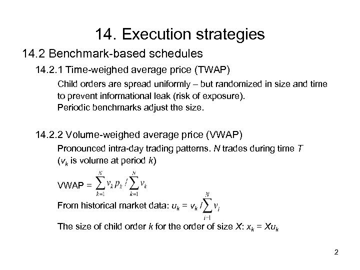14. Execution strategies 14. 2 Benchmark-based schedules 14. 2. 1 Time-weighed average price (TWAP) Child orders are spread uniformly – but randomized in size and time to prevent informational leak (risk of exposure). Periodic benchmarks adjust the size. 14. 2. 2 Volume-weighed average price (VWAP) Pronounced intra-day trading patterns. N trades during time T (νk is volume at period k) VWAP = From historical market data: uk = vk / The size of child order k for the order of size X: xk = Xuk 2

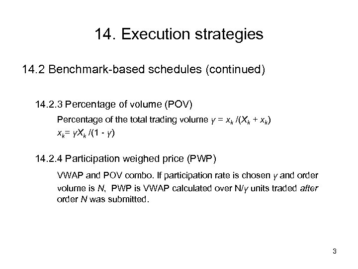14. Execution strategies 14. 2 Benchmark-based schedules (continued) 14. 2. 3 Percentage of volume (POV) Percentage of the total trading volume γ = xk /(Xk + xk) xk= γXk /(1 - γ) 14. 2. 4 Participation weighed price (PWP) VWAP and POV combo. If participation rate is chosen γ and order volume is N, PWP is VWAP calculated over N/γ units traded after order N was submitted. 3

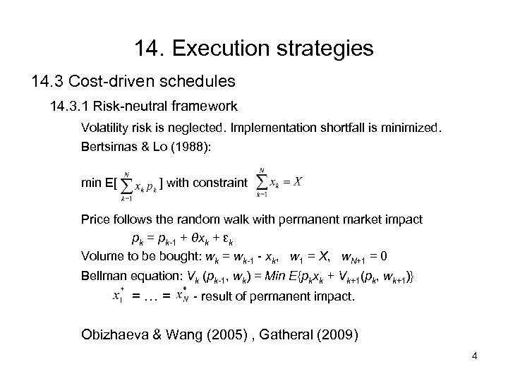14. Execution strategies 14. 3 Cost-driven schedules 14. 3. 1 Risk-neutral framework Volatility risk is neglected. Implementation shortfall is minimized. Bertsimas & Lo (1988): min E[ ] with constraint Price follows the random walk with permanent market impact pk = pk-1 + θxk + εk Volume to be bought: wk = wk-1 - xk, w 1 = X, w. N+1 = 0 Bellman equation: Vk (pk-1, wk) = Min E{pkxk + Vk+1(pk, wk+1)} =…= - result of permanent impact. Obizhaeva & Wang (2005) , Gatheral (2009) 4

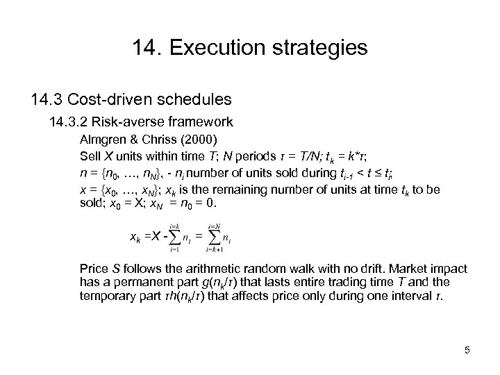14. Execution strategies 14. 3 Cost-driven schedules 14. 3. 2 Risk-averse framework Almgren & Chriss (2000) Sell X units within time T; N periods τ = T/N; tk = k*τ; n = {n 0, …, n. N}, - ni number of units sold during ti-1 < t ≤ ti; x = {x 0, …, x. N}; xk is the remaining number of units at time tk to be sold; x 0 = X; x. N = n 0 = 0. xk =X - = Price S follows the arithmetic random walk with no drift. Market impact has a permanent part g(nk/τ) that lasts entire trading time T and the temporary part τh(nk/τ) that affects price only during one interval τ. 5

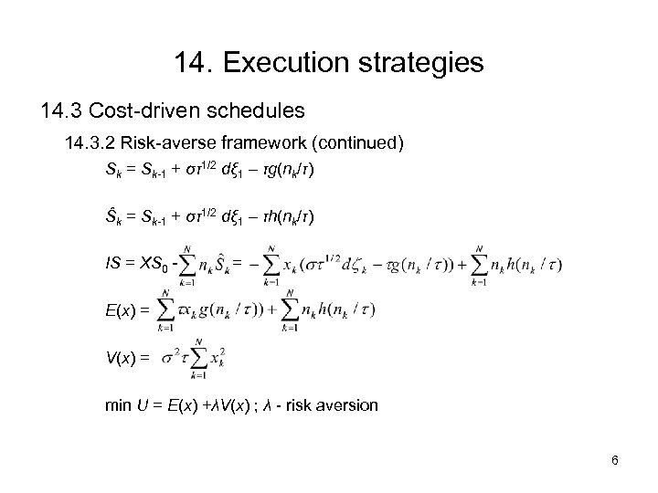14. Execution strategies 14. 3 Cost-driven schedules 14. 3. 2 Risk-averse framework (continued) Sk = Sk-1 + στ1/2 dξ 1 – τg(nk/τ) Ŝk = Sk-1 + στ1/2 dξ 1 – τh(nk/τ) IS = XS 0 - = E(x) = V(x) = min U = E(x) +λV(x) ; λ - risk aversion 6

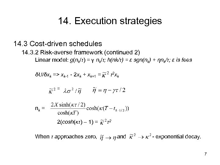14. Execution strategies 14. 3 Cost-driven schedules 14. 3. 2 Risk-averse framework (continued 2) Linear model: g(nk/τ) = γ nk/τ; h(nk/τ) = ε sgn(nk) + ηnk/τ; ε is fees δU/δxk => xk-1 - 2 xk + xk+1 = τ2 xk = nk = 2(cosh(κτ) – 1) = When τ approaches zero, τ2 and - exponential decay. 7

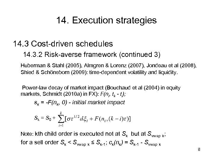14. Execution strategies 14. 3 Cost-driven schedules 14. 3. 2 Risk-averse framework (continued 3) Huberman & Stahl (2005), Almgren & Lorenz (2007), Jondeau et al (2008), Shied & Schöneborn (2009): time-dependent volatility and liquidity. Power-law decay of market impact (Bouchaud et al (2004) in equity markets, Schmidt (2010 a) in FX): F(ni, tk - ti); sk = -F(nk, 0) - initial market impact Sk = S 0 + Note: kth child order is executed not at Sk but at Svwap k; for a sell order Sk < Svwap k ≤ Sk-1; ck(nk) = Sk-1 - Svwap k 8

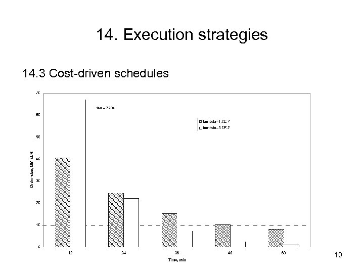
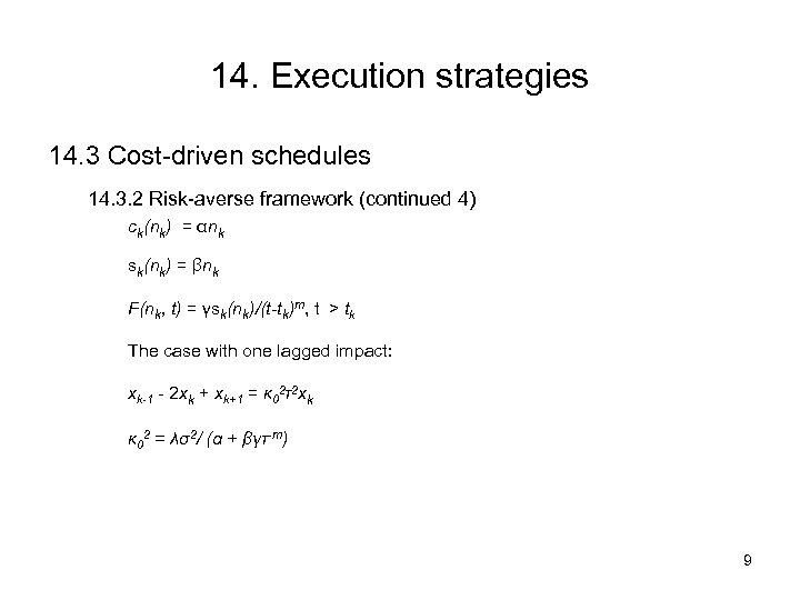14. Execution strategies 14. 3 Cost-driven schedules 14. 3. 2 Risk-averse framework (continued 4) ck(nk) = αnk sk(nk) = βnk F(nk, t) = γsk(nk)/(t-tk)m, t > tk The case with one lagged impact: xk-1 - 2 xk + xk+1 = κ 02τ2 xk κ 02 = λσ2/ (α + βγτ-m) 9

14. Execution strategies 14. 3 Cost-driven schedules 10

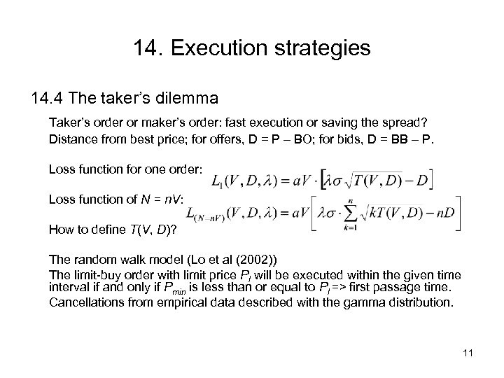14. Execution strategies 14. 4 The taker’s dilemma Taker’s order or maker’s order: fast execution or saving the spread? Distance from best price; for offers, D = P – BO; for bids, D = BB – P. Loss function for one order: Loss function of N = n. V: How to define T(V, D)? The random walk model (Lo et al (2002)) The limit-buy order with limit price Pl will be executed within the given time interval if and only if Pmin is less than or equal to Pl => first passage time. Cancellations from empirical data described with the gamma distribution. 11

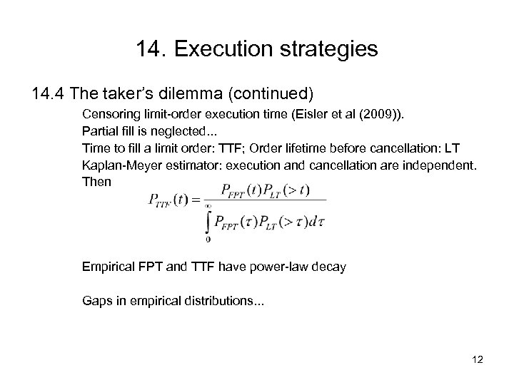14. Execution strategies 14. 4 The taker’s dilemma (continued) Censoring limit-order execution time (Eisler et al (2009)). Partial fill is neglected. . . Time to fill a limit order: TTF; Order lifetime before cancellation: LT Kaplan-Meyer estimator: execution and cancellation are independent. Then Empirical FPT and TTF have power-law decay Gaps in empirical distributions. . . 12

14. Execution strategies 14. 4 The taker’s dilemma – Simulations Input: • Best price - observable • Volume at best price - observable • Deal depletion rate – from simulations • Total depletion rate (deals + cancellations) – from simulations Output: • Expected loss • Expected execution time 13

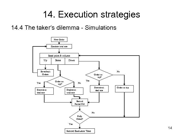14. Execution strategies 14. 4 The taker’s dilemma - Simulations New Order Simulate total rate Read price & volume Up Same Down No Re-submit Orders Yes Execute at deal rate Order on top? No Yes Execute at deal rate Deplete at total rate Order on top Record Partial Fill No Fully Filled? Yes Record Execution Time 14

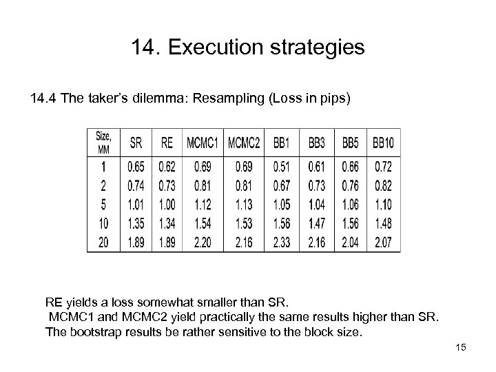14. Execution strategies 14. 4 The taker’s dilemma: Resampling (Loss in pips) RE yields a loss somewhat smaller than SR. MCMC 1 and MCMC 2 yield practically the same results higher than SR. The bootstrap results be rather sensitive to the block size. 15

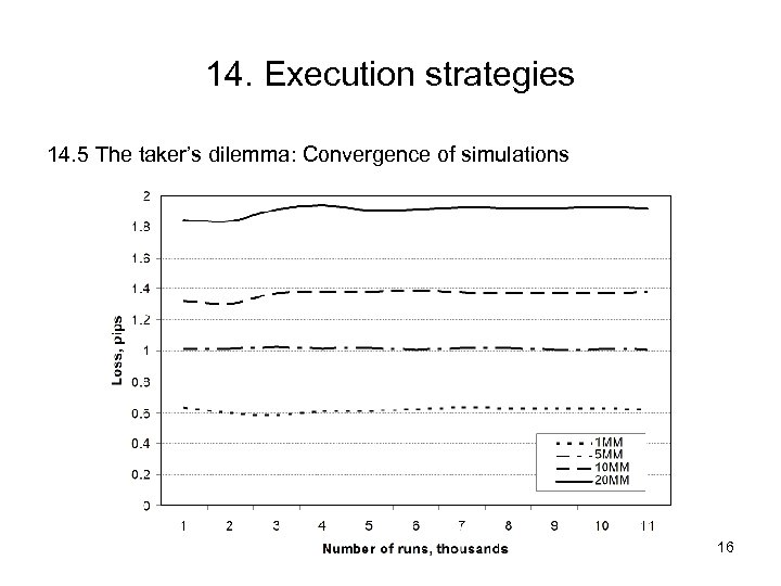14. Execution strategies 14. 5 The taker’s dilemma: Convergence of simulations 16

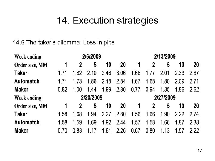14. Execution strategies 14. 6 The taker’s dilemma: Loss in pips 17

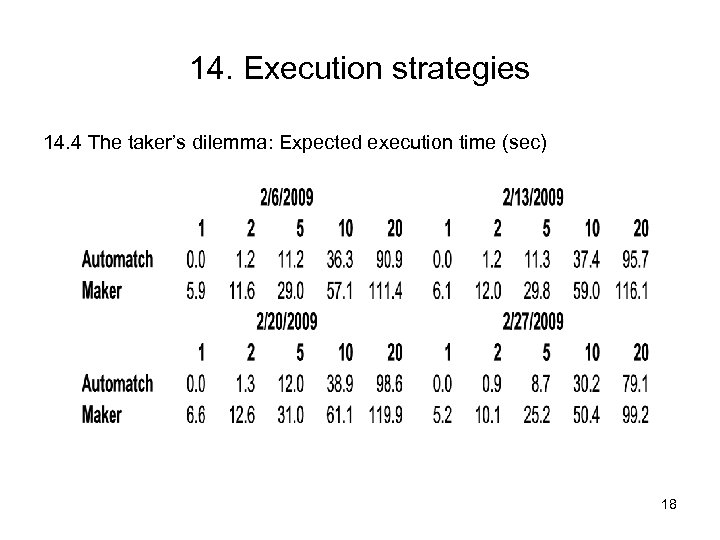14. Execution strategies 14. 4 The taker’s dilemma: Expected execution time (sec) 18