12 Models of limit-order markets 12 1 Cohen

12. Models of limit-order markets 12. 1 Cohen, Maier, Schwartz, and Whitcomb (1981) - Traders maximize their wealth that consists of cash and a risky asset. - Traders trade only at a set of fixed points of time. - Trading costs include a fee for submitting a limit order and a another fee paid in case an order is filled. - Trading is symmetric on both sides of the market. - Price follows random walk with shocks summed up between trading according to the compound Poisson process ln St(Δ) = ln St + Δ - time between trading points, price shocks Zi are IID with zero mean N(Δ) is a Poisson process with arrival rate ν. 1

12. Models of limit-order markets 12. 1 CMSW (continued) Trader’s choice: - not to trade - market buy - bid at a price lower than current ask Probability to fill a limit order is always less than unity First passage time (FPT): S(t=0) = S 0. FPT for shock s is the time t of the first instance when S(t) <= S 0 - s. f. FPT(s, t) = ~ t-3/2 Expected time is infinite. 2

12. Models of limit-order markets 12. 1 CMSW (continued 2) Dynamic programming problem of maximizing trader’s wealth. In the CMSW model, the bid/ask spread is determined with transaction costs. If the spread is wide, traders submit new limit orders that have lower spread but still have lower loss than market orders. When the spread narrows to the extent that fees for submitting limit orders negate their gain, traders may want to submit market orders (“gravitational pull”). Order matching widens the spread as market orders “wipe out” top of the book. Ultimately the spread attains some equilibrium value. Market thickness is defined with order arrival rate. The spread increases as the market becomes “thinner”. 3

12. Models of limit-order markets 12. 2 The Parlour model (1998) - Risk-neutral traders perceive asset value as vβ(t); v – fundamental value; β(t) randomly distributed within [ , ]. - Exogenous bid (B) and ask (A) prices + active LOB with n. A(t) and n. B(t) - One trader at a time trades one unit of asset at times t = 1, . . . , T. - Buy or Sell with probability 0. 5. - Buyer: If vβ(t) > A: n. A(t+1) = n. A(t) – 1; else: n. B(t+1) = n. B(t) + 1. - Seller: If vβ(t) < B: n. B(t+1) = n. B(t) – 1; else: n. A(t+1) = n. A(t) + 1. Optimal solution depends on the history. Hence backward recursion. The last trader (T) does not submit limit orders. Hence the change in active LOB is known at time T. Then the action of trader T-1 is determined, etc. 4

12. Models of limit-order markets 12. 2 The Parlour model (continued) The outcome coincides with empirical findings: Market orders are more likely submitted after market orders on the same side of the market. Indeed, one may expect that a buy order diminishes liquidity on the ask side, which motivates a seller to submit a limit ask order. Buyer (seller) is more likely to submit a market order in case of a thick LOB on the bid (ask) side. On the other hand, a thick LOB on the offer (bid) side motivates a buyer (seller) to submit a limit order. 5

12. Models of limit-order markets 12. 3 The Foucault model (1999) Winner’s curse: the highest bid and lowest offer “picked off” by market orders may be mispriced. - One trader at a time trades one unit of asset at times t = 1, . . . , T. - Trading can stop at any time with Pr = 1 - ρ - Asset value follows random walk: v(t) = v(t-1) + ε(t); ε(t) = ±σ with Pr = 0. 5. - Trader’s estimate of asset value: R(t) = v(t) + y(t); y(t) = ±L with Pr = 0. 5. - Trader may submit buy or sell, market or limit order. - Limit orders live one period, then they are cancelled. - If bid side is empty, B(t) = -∞; if the ask side is empty, A(t) = ∞, and trader posts orders on both sides of the market. 6

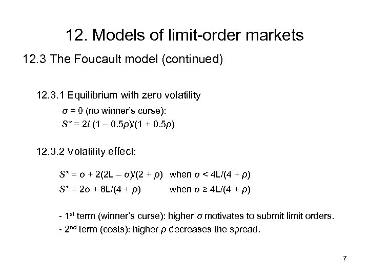12. Models of limit-order markets 12. 3 The Foucault model (continued) 12. 3. 1 Equilibrium with zero volatility σ = 0 (no winner’s curse): S* = 2 L(1 – 0. 5ρ)/(1 + 0. 5ρ) 12. 3. 2 Volatility effect: S* = σ + 2(2 L – σ)/(2 + ρ) when σ < 4 L/(4 + ρ) S* = 2σ + 8 L/(4 + ρ) when σ ≥ 4 L/(4 + ρ) - 1 st term (winner’s curse): higher σ motivates to submit limit orders. - 2 nd term (costs): higher ρ decreases the spread. 7

12. Models of limit-order markets 12. 4 Summary • • Thinner LOB has a wider spread. Market orders are more likely submitted after market orders on the same side of LOB. Buyer (seller) is more likely to submit market order in case of thick LOB on the bid (ask) side. Buyer (seller) is more likely to submit limit order in case of thick LOB on the ask (bid) side. The spread increases with volatility. Winner’s curse occurs when a limit order filled due to price volatility turns out to be mispriced. Patient traders submit less aggressive limit orders, which increases the spread. Limit orders can cluster outside the market, generating a hump-shaped LOB. 8