11 -755 Machine Learning for Signal Processing Eigen

11 -755 Machine Learning for Signal Processing Eigen Representations: Detecting faces in images Class 6. 15 Sep 2011 Instructor: Bhiksha Raj

Administrivia Project teams? Project proposals? TAs have updated timings and locations (on webpage) 11 -755 MLSP: Bhiksha Raj

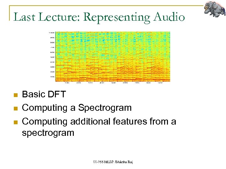Last Lecture: Representing Audio Basic DFT Computing a Spectrogram Computing additional features from a spectrogram 11 -755 MLSP: Bhiksha Raj

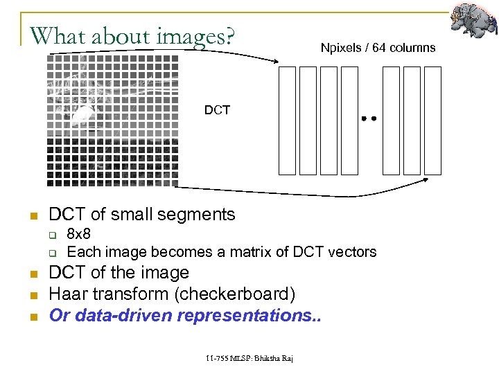What about images? Npixels / 64 columns DCT of small segments q q 8 x 8 Each image becomes a matrix of DCT vectors DCT of the image Haar transform (checkerboard) Or data-driven representations. . 11 -755 MLSP: Bhiksha Raj

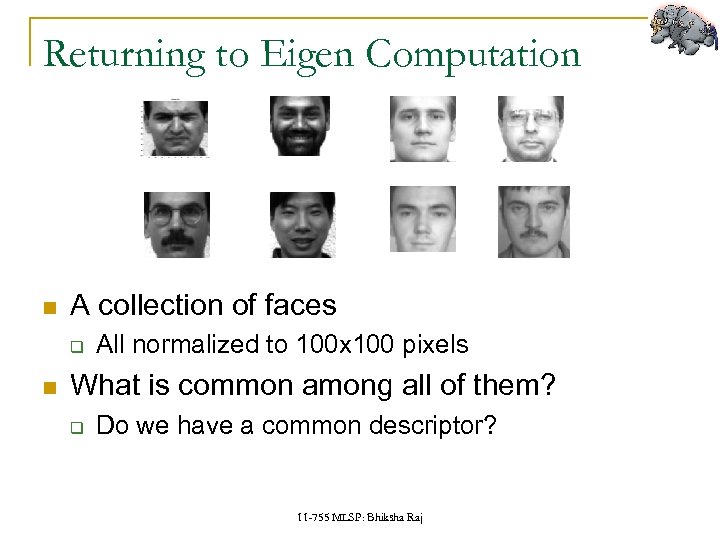Returning to Eigen Computation A collection of faces q All normalized to 100 x 100 pixels What is common among all of them? q Do we have a common descriptor? 11 -755 MLSP: Bhiksha Raj

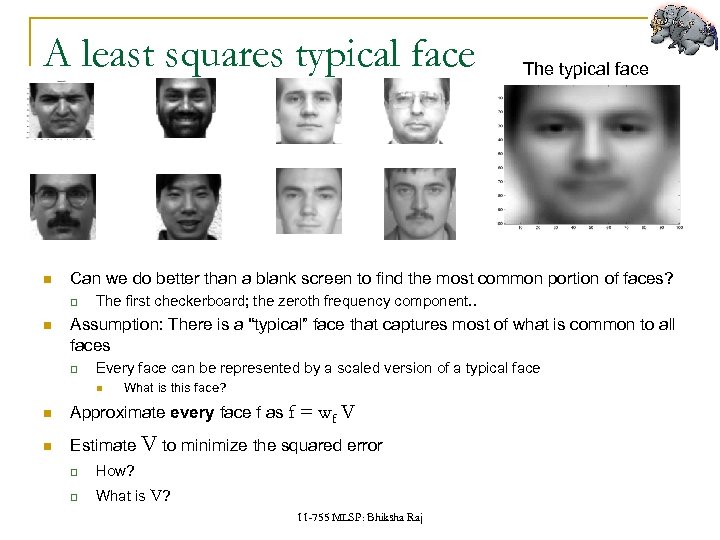A least squares typical face Can we do better than a blank screen to find the most common portion of faces? q The typical face The first checkerboard; the zeroth frequency component. . Assumption: There is a “typical” face that captures most of what is common to all faces q Every face can be represented by a scaled version of a typical face What is this face? Approximate every face f as f = wf V Estimate V to minimize the squared error q How? q What is V? 11 -755 MLSP: Bhiksha Raj

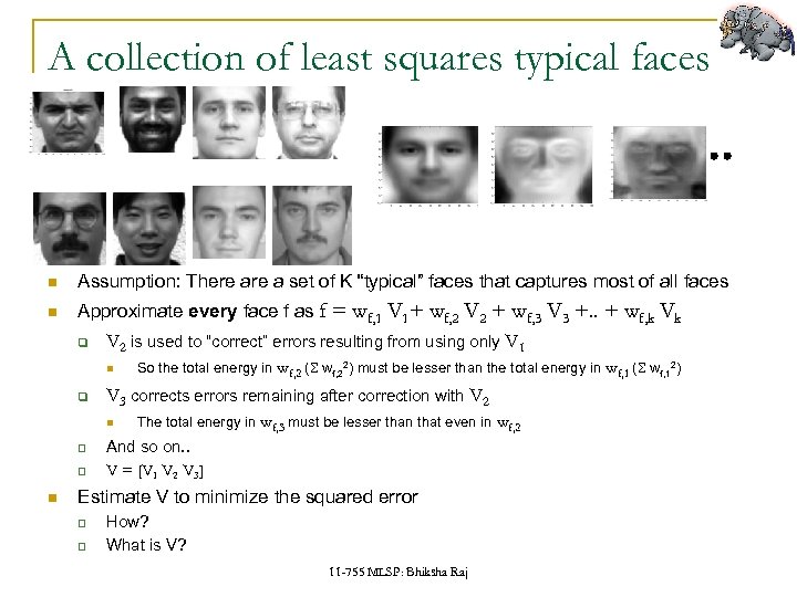A collection of least squares typical faces Assumption: There a set of K “typical” faces that captures most of all faces Approximate every face f as f = wf, 1 V 1+ wf, 2 V 2 + wf, 3 V 3 +. . + wf, k Vk q V 2 is used to “correct” errors resulting from using only V 1 q q wf, 2 (S wf, 22) must be lesser than the total energy in wf, 1 (S wf, 12) V 3 corrects errors remaining after correction with V 2 q So the total energy in The total energy in wf, 3 must be lesser than that even in wf, 2 And so on. . V = [V 1 V 2 V 3] Estimate V to minimize the squared error q q How? What is V? 11 -755 MLSP: Bhiksha Raj

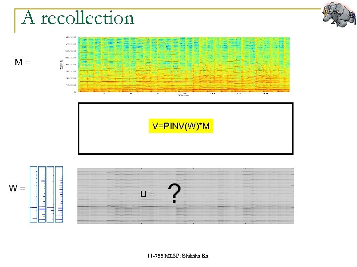A recollection M= V=PINV(W)*M W= U= ? 11 -755 MLSP: Bhiksha Raj

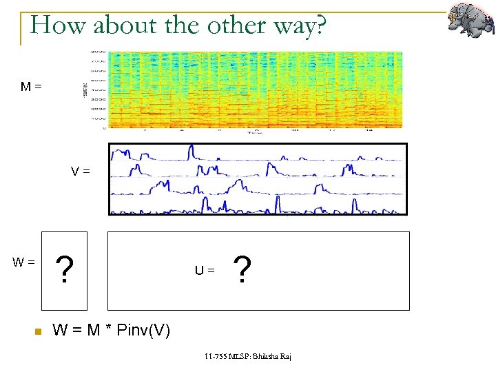How about the other way? M= V= W= ? U= ? W = M * Pinv(V) 11 -755 MLSP: Bhiksha Raj

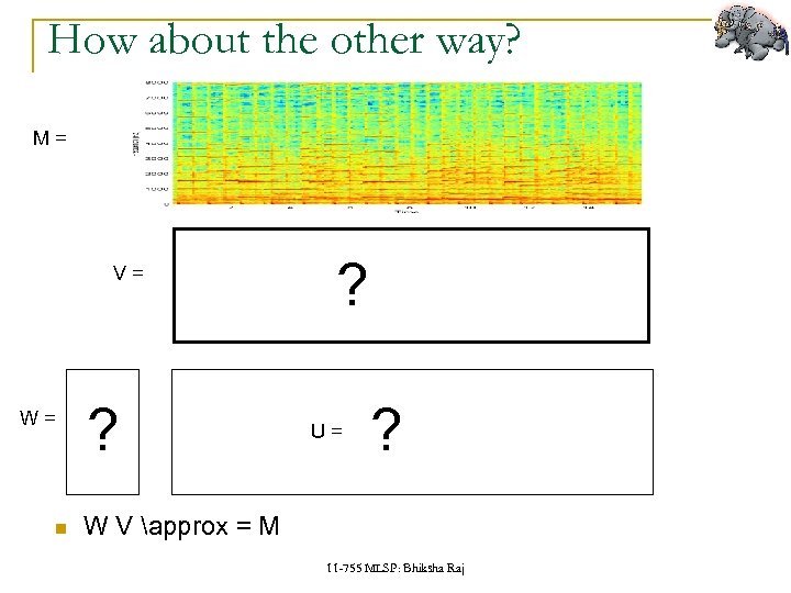How about the other way? M= V= W= ? ? U= ? W V approx = M 11 -755 MLSP: Bhiksha Raj

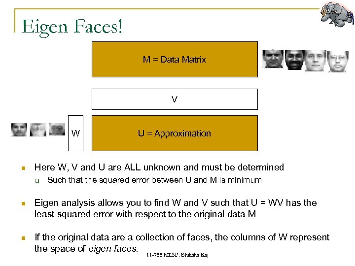Eigen Faces! M = Data Matrix V W U = Approximation Here W, V and U are ALL unknown and must be determined q Such that the squared error between U and M is minimum Eigen analysis allows you to find W and V such that U = WV has the least squared error with respect to the original data M If the original data are a collection of faces, the columns of W represent the space of eigen faces. 11 -755 MLSP: Bhiksha Raj

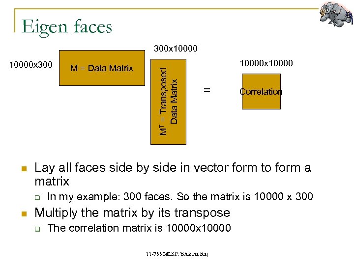Eigen faces 10000 x 300 10000 x 10000 = Correlation Lay all faces side by side in vector form to form a matrix q M = Data Matrix MT = Transposed Data Matrix 300 x 10000 In my example: 300 faces. So the matrix is 10000 x 300 Multiply the matrix by its transpose q The correlation matrix is 10000 x 10000 11 -755 MLSP: Bhiksha Raj

Eigen faces eigenface 1 eigenface 2 [U, S] = eig(correlation) Compute the eigen vectors q Only 300 of the 10000 eigen values are non-zero Why? Retain eigen vectors with high eigen values (>0) q Could use a higher threshold 11 -755 MLSP: Bhiksha Raj

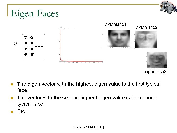Eigen Faces eigenface 2 eigenface 1 eigenface 3 The eigen vector with the highest eigen value is the first typical face The vector with the second highest eigen value is the second typical face. Etc. 11 -755 MLSP: Bhiksha Raj

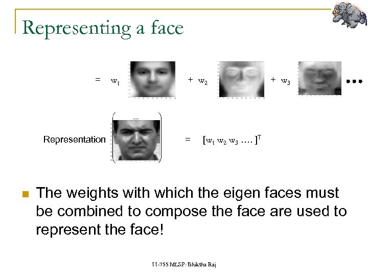Representing a face = Representation w 1 + w 2 = + w 3 [w 1 w 2 w 3 …. ]T The weights with which the eigen faces must be combined to compose the face are used to represent the face! 11 -755 MLSP: Bhiksha Raj

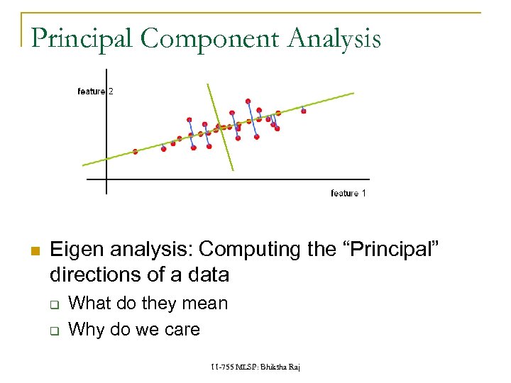Principal Component Analysis Eigen analysis: Computing the “Principal” directions of a data q q What do they mean Why do we care 11 -755 MLSP: Bhiksha Raj

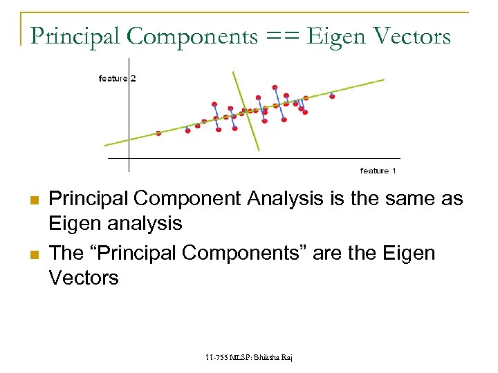Principal Components == Eigen Vectors Principal Component Analysis is the same as Eigen analysis The “Principal Components” are the Eigen Vectors 11 -755 MLSP: Bhiksha Raj

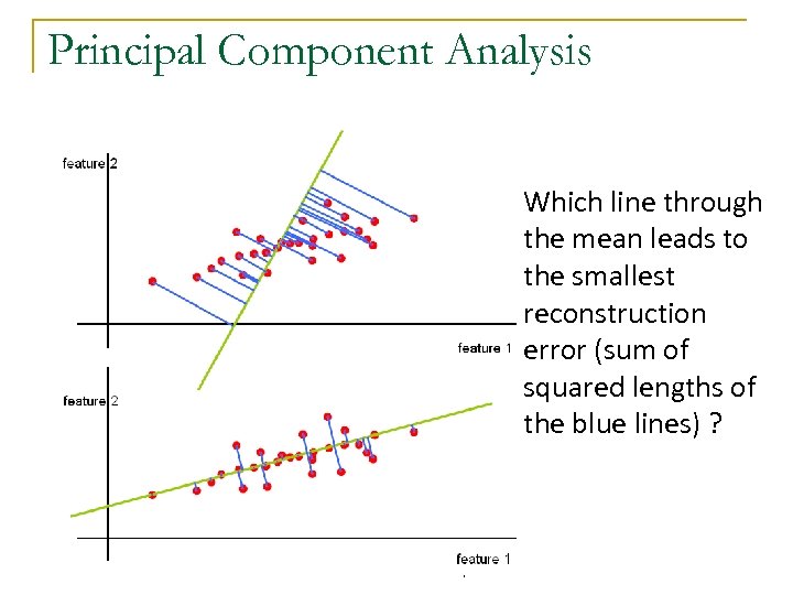Principal Component Analysis Which line through the mean leads to the smallest reconstruction error (sum of squared lengths of the blue lines) ? 11 -755 MLSP: Bhiksha Raj

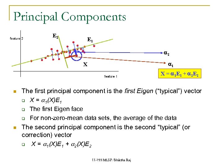Principal Components E 2 E 1 a 2 a 1 X X = a 1 E 1 + a 2 E 2 The first principal component is the first Eigen (“typical”) vector q X = a 1(X)E 1 q The first Eigen face q For non-zero-mean data sets, the average of the data The second principal component is the second “typical” (or correction) vector q X = a 1(X)E 1 + a 2(X)E 2 11 -755 MLSP: Bhiksha Raj

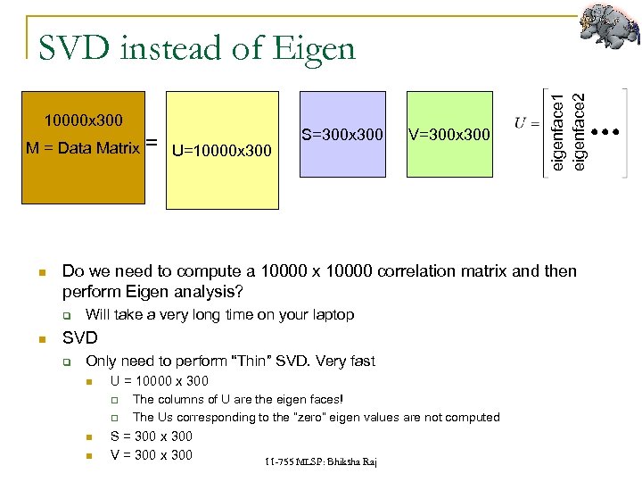10000 x 300 M = Data Matrix U=10000 x 300 S=300 x 300 V=300 x 300 Do we need to compute a 10000 x 10000 correlation matrix and then perform Eigen analysis? q = eigenface 1 eigenface 2 SVD instead of Eigen Will take a very long time on your laptop SVD q Only need to perform “Thin” SVD. Very fast U = 10000 x 300 q q The columns of U are the eigen faces! The Us corresponding to the “zero” eigen values are not computed S = 300 x 300 V = 300 x 300 11 -755 MLSP: Bhiksha Raj

NORMALIZING OUT VARIATIONS 11 -755 MLSP: Bhiksha Raj

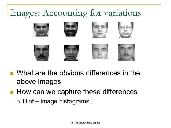Images: Accounting for variations What are the obvious differences in the above images How can we capture these differences q Hint – image histograms. . 11 -755 MLSP: Bhiksha Raj

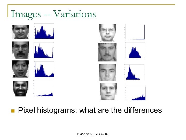Images -- Variations Pixel histograms: what are the differences 11 -755 MLSP: Bhiksha Raj

Normalizing Image Characteristics Normalize the pictures q Eliminate lighting/contrast variations q All pictures must have “similar” lighting How? Lighting and contrast are represented in the image histograms: 11 -755 MLSP: Bhiksha Raj

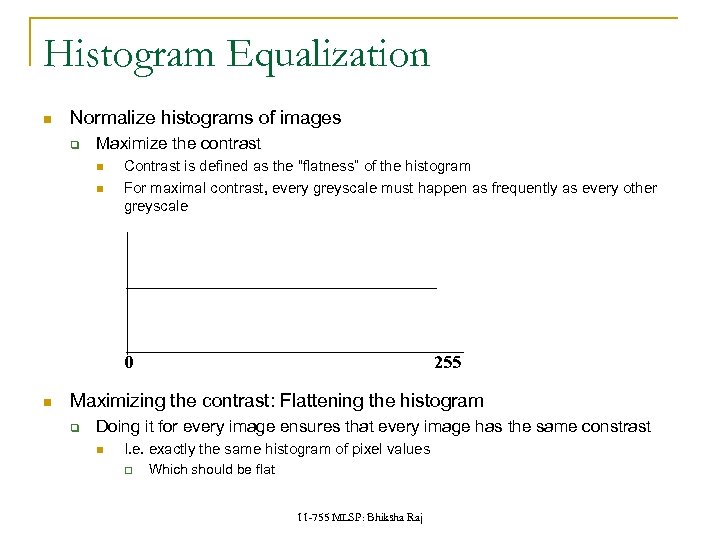Histogram Equalization Normalize histograms of images q Maximize the contrast Contrast is defined as the “flatness” of the histogram For maximal contrast, every greyscale must happen as frequently as every other greyscale 0 255 Maximizing the contrast: Flattening the histogram q Doing it for every image ensures that every image has the same constrast I. e. exactly the same histogram of pixel values q Which should be flat 11 -755 MLSP: Bhiksha Raj

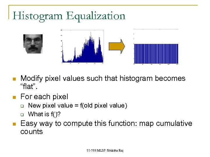Histogram Equalization Modify pixel values such that histogram becomes “flat”. For each pixel q q New pixel value = f(old pixel value) What is f()? Easy way to compute this function: map cumulative counts 11 -755 MLSP: Bhiksha Raj

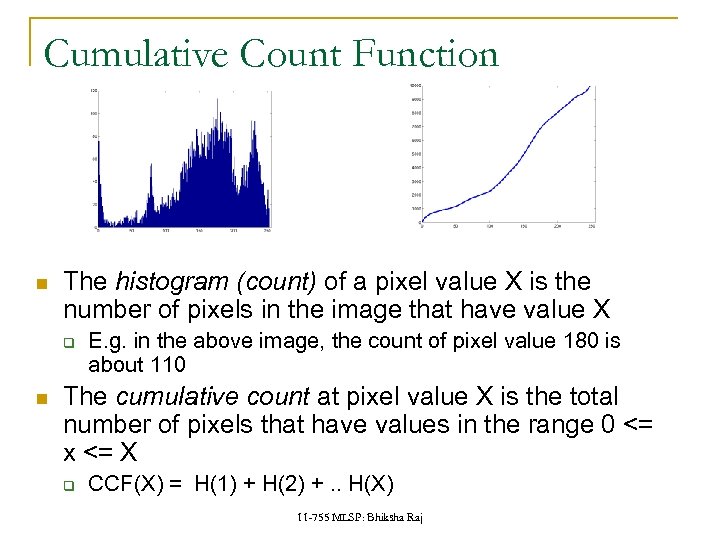Cumulative Count Function The histogram (count) of a pixel value X is the number of pixels in the image that have value X q E. g. in the above image, the count of pixel value 180 is about 110 The cumulative count at pixel value X is the total number of pixels that have values in the range 0 <= x <= X q CCF(X) = H(1) + H(2) +. . H(X) 11 -755 MLSP: Bhiksha Raj

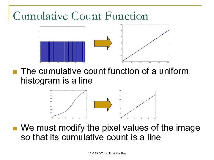Cumulative Count Function The cumulative count function of a uniform histogram is a line We must modify the pixel values of the image so that its cumulative count is a line 11 -755 MLSP: Bhiksha Raj

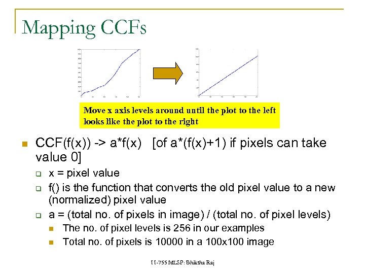Mapping CCFs Move x axis levels around until the plot to the left looks like the plot to the right CCF(f(x)) -> a*f(x) [of a*(f(x)+1) if pixels can take value 0] q q q x = pixel value f() is the function that converts the old pixel value to a new (normalized) pixel value a = (total no. of pixels in image) / (total no. of pixel levels) The no. of pixel levels is 256 in our examples Total no. of pixels is 10000 in a 100 x 100 image 11 -755 MLSP: Bhiksha Raj

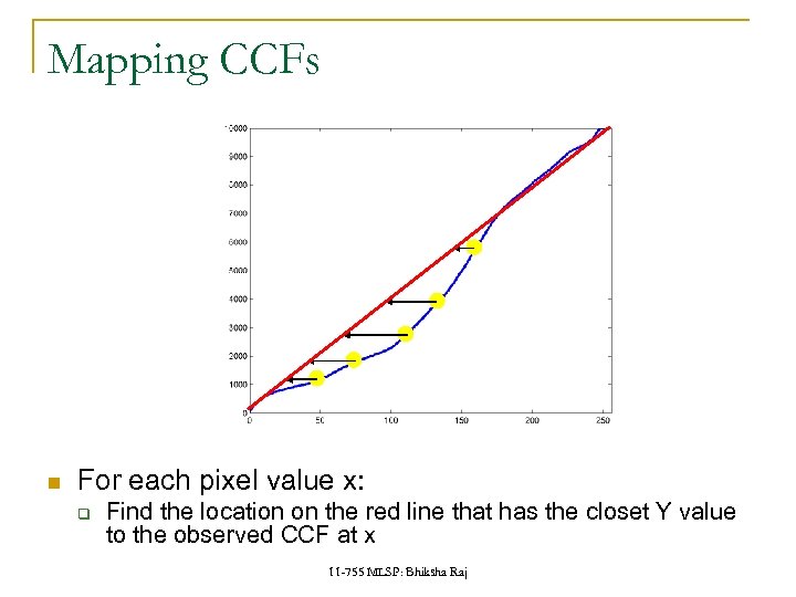Mapping CCFs For each pixel value x: q Find the location on the red line that has the closet Y value to the observed CCF at x 11 -755 MLSP: Bhiksha Raj

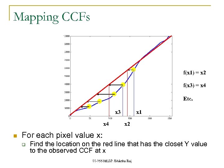Mapping CCFs f(x 1) = x 2 f(x 3) = x 4 Etc. x 3 x 4 x 1 x 2 For each pixel value x: q Find the location on the red line that has the closet Y value to the observed CCF at x 11 -755 MLSP: Bhiksha Raj

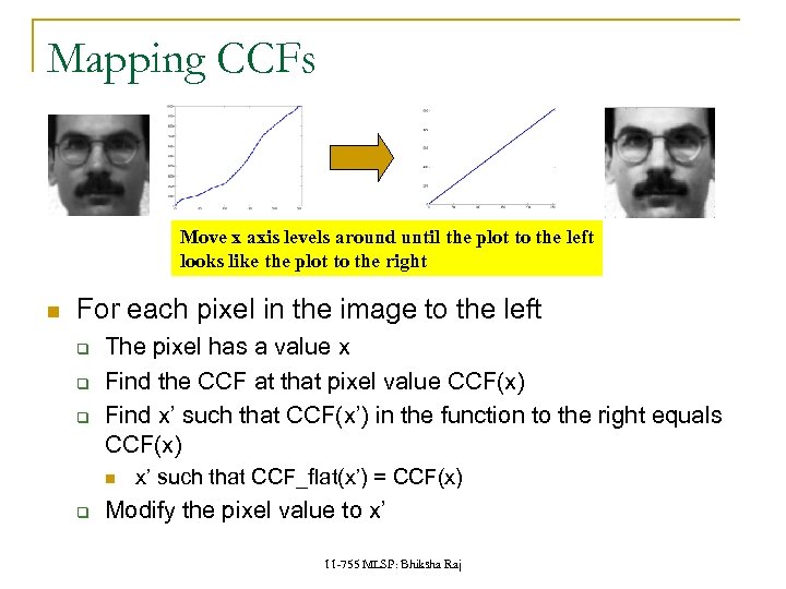Mapping CCFs Move x axis levels around until the plot to the left looks like the plot to the right For each pixel in the image to the left q q q The pixel has a value x Find the CCF at that pixel value CCF(x) Find x’ such that CCF(x’) in the function to the right equals CCF(x) q x’ such that CCF_flat(x’) = CCF(x) Modify the pixel value to x’ 11 -755 MLSP: Bhiksha Raj

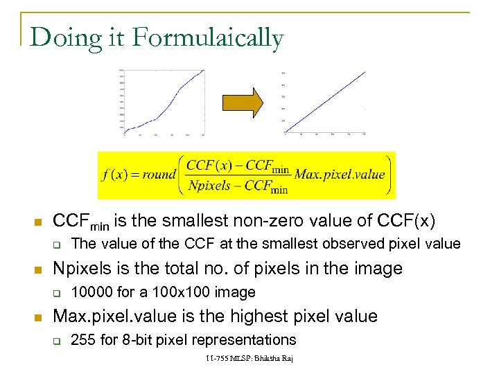Doing it Formulaically CCFmin is the smallest non-zero value of CCF(x) q Npixels is the total no. of pixels in the image q The value of the CCF at the smallest observed pixel value 10000 for a 100 x 100 image Max. pixel. value is the highest pixel value q 255 for 8 -bit pixel representations 11 -755 MLSP: Bhiksha Raj

Or even simpler Matlab: q Newimage = histeq(oldimage) 11 -755 MLSP: Bhiksha Raj

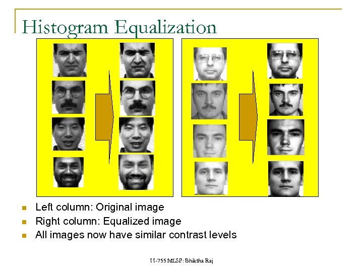Histogram Equalization Left column: Original image Right column: Equalized image All images now have similar contrast levels 11 -755 MLSP: Bhiksha Raj

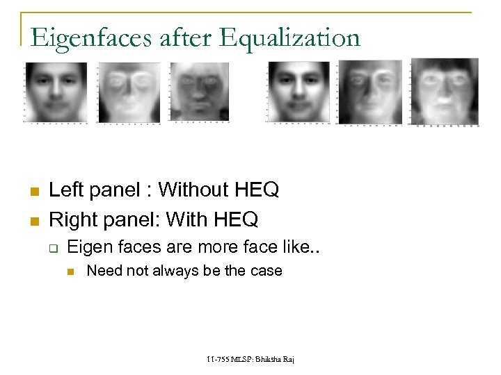Eigenfaces after Equalization Left panel : Without HEQ Right panel: With HEQ q Eigen faces are more face like. . Need not always be the case 11 -755 MLSP: Bhiksha Raj

Detecting Faces in Images 11 -755 MLSP: Bhiksha Raj

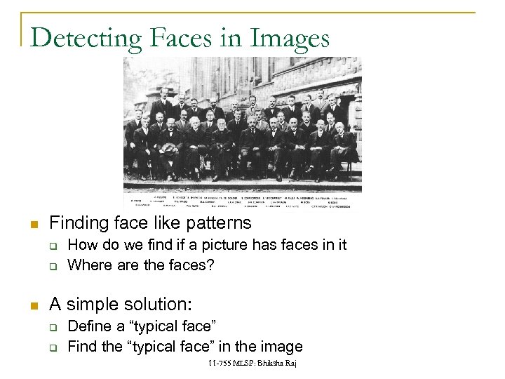Detecting Faces in Images Finding face like patterns q q How do we find if a picture has faces in it Where are the faces? A simple solution: q q Define a “typical face” Find the “typical face” in the image 11 -755 MLSP: Bhiksha Raj

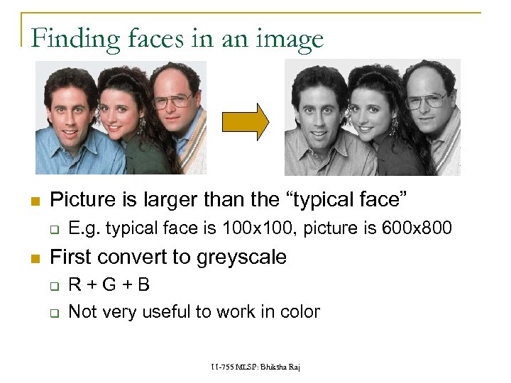Finding faces in an image Picture is larger than the “typical face” q E. g. typical face is 100 x 100, picture is 600 x 800 First convert to greyscale q q R+G+B Not very useful to work in color 11 -755 MLSP: Bhiksha Raj

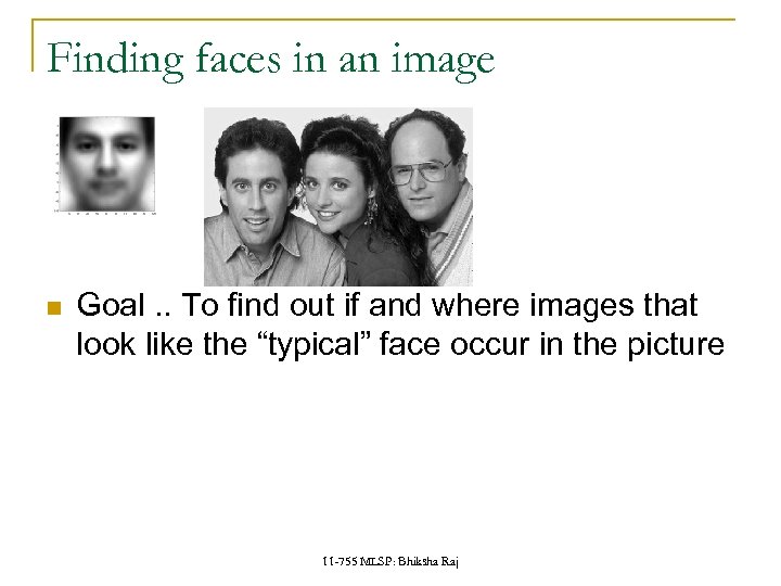Finding faces in an image Goal. . To find out if and where images that look like the “typical” face occur in the picture 11 -755 MLSP: Bhiksha Raj

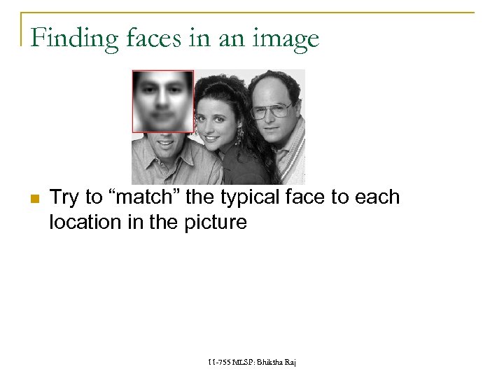Finding faces in an image Try to “match” the typical face to each location in the picture 11 -755 MLSP: Bhiksha Raj

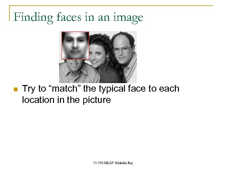Finding faces in an image Try to “match” the typical face to each location in the picture 11 -755 MLSP: Bhiksha Raj

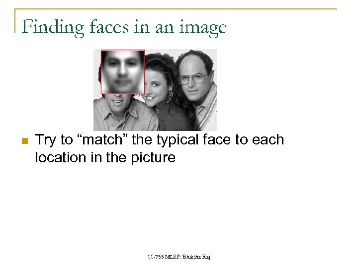Finding faces in an image Try to “match” the typical face to each location in the picture 11 -755 MLSP: Bhiksha Raj

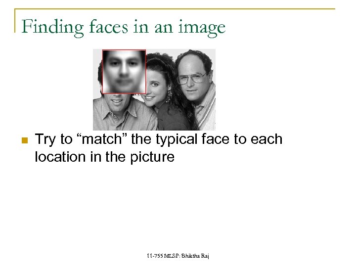Finding faces in an image Try to “match” the typical face to each location in the picture 11 -755 MLSP: Bhiksha Raj

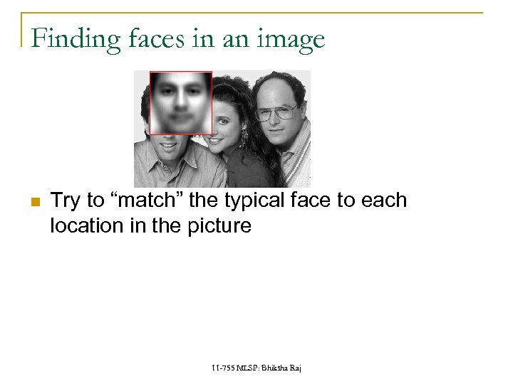Finding faces in an image Try to “match” the typical face to each location in the picture 11 -755 MLSP: Bhiksha Raj

Finding faces in an image Try to “match” the typical face to each location in the picture 11 -755 MLSP: Bhiksha Raj

Finding faces in an image Try to “match” the typical face to each location in the picture 11 -755 MLSP: Bhiksha Raj

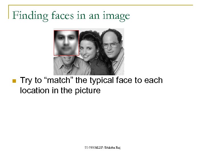Finding faces in an image Try to “match” the typical face to each location in the picture 11 -755 MLSP: Bhiksha Raj

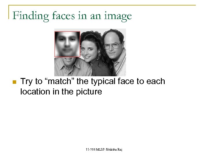Finding faces in an image Try to “match” the typical face to each location in the picture 11 -755 MLSP: Bhiksha Raj

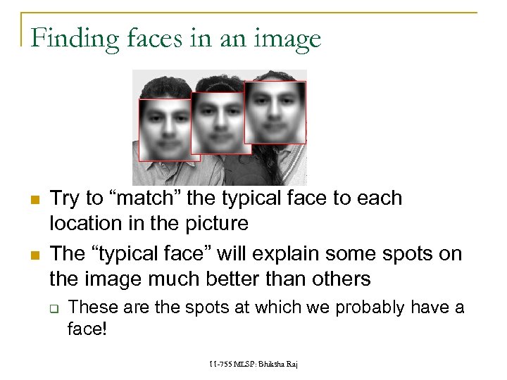Finding faces in an image Try to “match” the typical face to each location in the picture The “typical face” will explain some spots on the image much better than others q These are the spots at which we probably have a face! 11 -755 MLSP: Bhiksha Raj

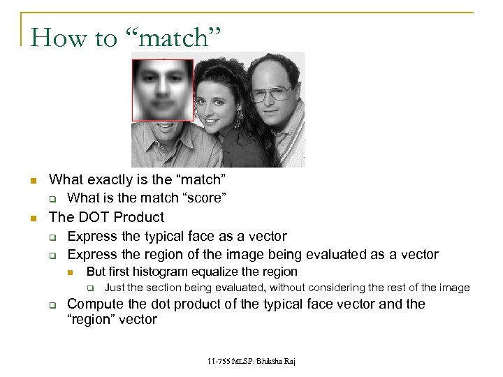How to “match” What exactly is the “match” q What is the match “score” The DOT Product q Express the typical face as a vector q Express the region of the image being evaluated as a vector But first histogram equalize the region q q Just the section being evaluated, without considering the rest of the image Compute the dot product of the typical face vector and the “region” vector 11 -755 MLSP: Bhiksha Raj

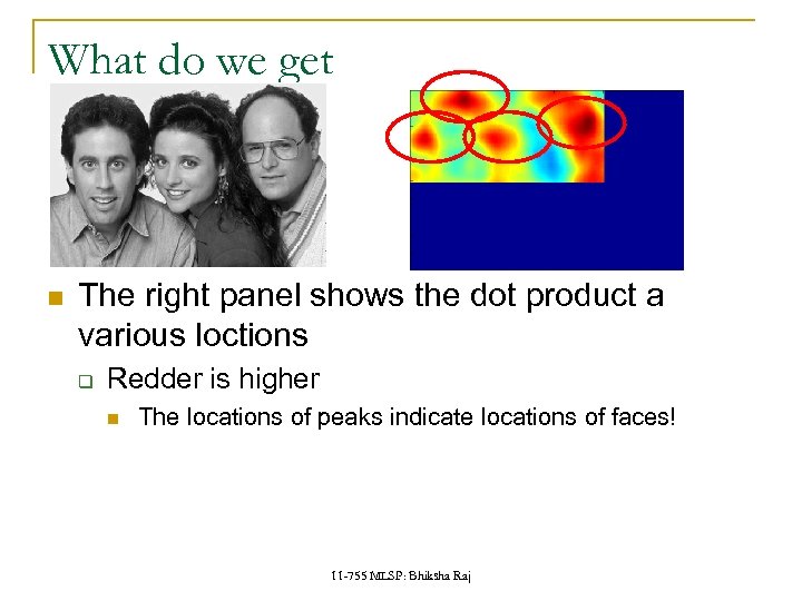What do we get The right panel shows the dot product a various loctions q Redder is higher The locations of peaks indicate locations of faces! 11 -755 MLSP: Bhiksha Raj

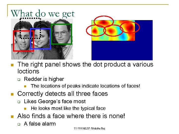What do we get The right panel shows the dot product a various loctions q Redder is higher Correctly detects all three faces q Likes George’s face most The locations of peaks indicate locations of faces! He looks most like the typical face Also finds a face where there is none! q A false alarm 11 -755 MLSP: Bhiksha Raj

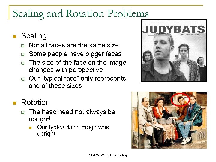Scaling and Rotation Problems Scaling q q Not all faces are the same size Some people have bigger faces The size of the face on the image changes with perspective Our “typical face” only represents one of these sizes Rotation q The head need not always be upright! Our typical face image was upright 11 -755 MLSP: Bhiksha Raj

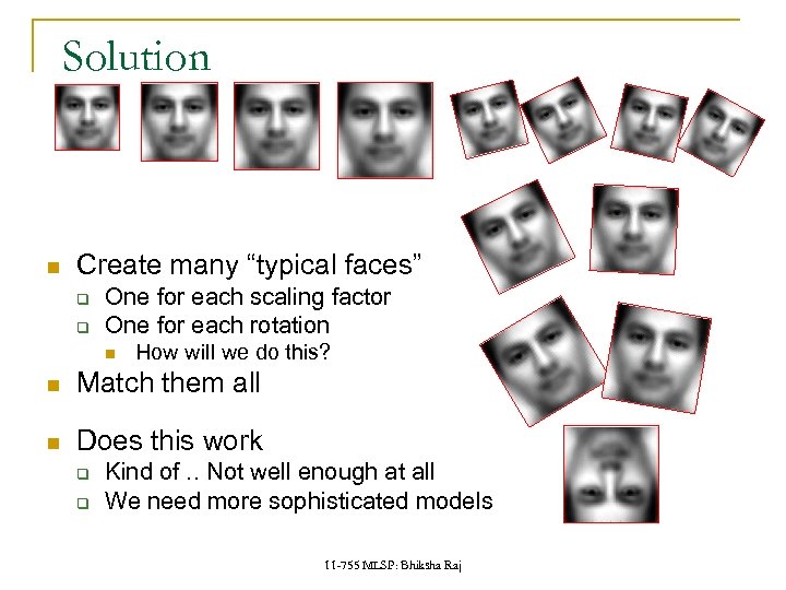Solution Create many “typical faces” q q One for each scaling factor One for each rotation How will we do this? Match them all Does this work q q Kind of. . Not well enough at all We need more sophisticated models 11 -755 MLSP: Bhiksha Raj

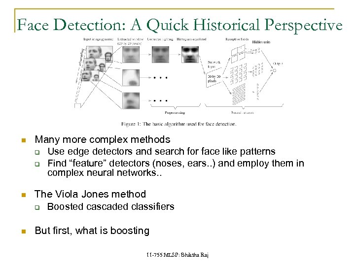Face Detection: A Quick Historical Perspective Many more complex methods q Use edge detectors and search for face like patterns q Find “feature” detectors (noses, ears. . ) and employ them in complex neural networks. . The Viola Jones method q Boosted cascaded classifiers But first, what is boosting 11 -755 MLSP: Bhiksha Raj

And even before that – what is classification? Given “features” describing an entity, determine the category it belongs to q Walks on two legs, has no hair. Is this q Has long hair, is 5’ 4” tall, is this q A Chimpanizee A Human A woman Matches “eye” pattern with score 0. 5, “mouth pattern” with score 0. 25, “nose” pattern with score 0. 1. Are we looking at A face Not a face? 11 -755 MLSP: Bhiksha Raj

Classification Multi-classification q Many possible categories Binary classification q Only two categories E. g. Sounds “AH, IY, UW, EY. . ” E. g. Images “Tree, dog, house, person. . ” Man vs. Woman Face vs. not a face. . Face detection: Recast as binary face classification q For each little square of the image, determine if the square represents a face or not 11 -755 MLSP: Bhiksha Raj

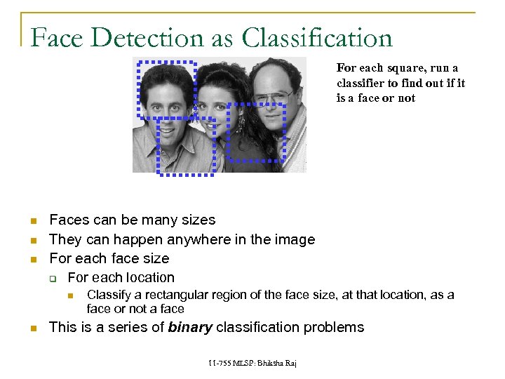Face Detection as Classification For each square, run a classifier to find out if it is a face or not Faces can be many sizes They can happen anywhere in the image For each face size q For each location Classify a rectangular region of the face size, at that location, as a face or not a face This is a series of binary classification problems 11 -755 MLSP: Bhiksha Raj

Introduction to Boosting An ensemble method that sequentially combines many simple BINARY classifiers to construct a final complex classifier q q Each weak learner focuses on instances where the previous classifier failed q Give greater weight to instances that have been incorrectly classified by previous learners Restrictions for weak learners q Simple classifiers are often called “weak” learners The complex classifiers are called “strong” learners Better than 50% correct Final classifier is weighted sum of weak classifiers 11 -755 MLSP: Bhiksha Raj

Boosting: A very simple idea One can come up with many rules to classify q E. g. Chimpanzee vs. Human classifier: q If arms == long, entity is chimpanzee q If height > 5’ 6” entity is human q If lives in house == entity is human q If lives in zoo == entity is chimpanzee Each of them is a reasonable rule, but makes many mistakes q Each rule has an intrinsic error rate Combine the predictions of these rules q But not equally q Rules that are less accurate should be given lesser weight 11 -755 MLSP: Bhiksha Raj

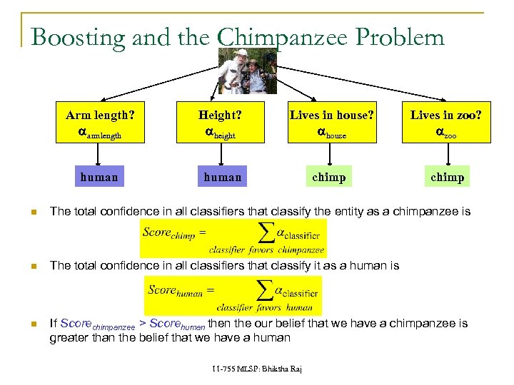Boosting and the Chimpanzee Problem Arm length? aarmlength Height? aheight Lives in house? ahouse Lives in zoo? azoo human chimp The total confidence in all classifiers that classify the entity as a chimpanzee is The total confidence in all classifiers that classify it as a human is If Scorechimpanzee > Scorehuman the our belief that we have a chimpanzee is greater than the belief that we have a human 11 -755 MLSP: Bhiksha Raj

Boosting as defined by Freund A gambler wants to write a program to predict winning horses. His program must encode the expertise of his brilliant winner friend The friend has no single, encodable algorithm. Instead he has many rules of thumb q He uses a different rule of thumb for each set of races q But cannot really enumerate what rules of thumbs go with what sets of races: he simply “knows” when he encounters a set E. g. “in this set, go with races that have black horses with stars on their foreheads” A common problem that faces us in many situations Problem: q q How best to combine all of the friend’s rules of thumb What is the best set of races to present to the friend, to extract the various rules of thumb 11 -755 MLSP: Bhiksha Raj

Boosting The basic idea: Can a “weak” learning algorithm that performs just slightly better than random guessing be boosted into an arbitrarily accurate “strong” learner q Each of the gambler’s rules may be just better than random guessing This is a “meta” algorithm, that poses no constraints on the form of the weak learners themselves q The gambler’s rules of thumb can be anything 11 -755 MLSP: Bhiksha Raj

Boosting: A Voting Perspective Boosting can be considered a form of voting q q q Let a number of different classifiers classify the data Go with the majority Intuition says that as the number of classifiers increases, the dependability of the majority vote increases The corresponding algorithms were called Boosting by majority q q q A (weighted) majority vote taken over all the classifiers How do we compute weights for the classifiers? How do we actually train the classifiers 11 -755 MLSP: Bhiksha Raj

ADA Boost: Adaptive algorithm for learning the weights ADA Boost: Not named of ADA Lovelace An adaptive algorithm that learns the weights of each classifier sequentially q Learning adapts to the current accuracy Iteratively: q Train a simple classifier from training data It will make errors even on training data Train a new classifier that focuses on the training data points that have been misclassified 11 -755 MLSP: Bhiksha Raj

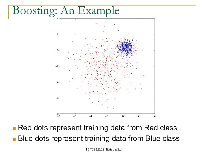Boosting: An Example Red dots represent training data from Red class Blue dots represent training data from Blue class 11 -755 MLSP: Bhiksha Raj

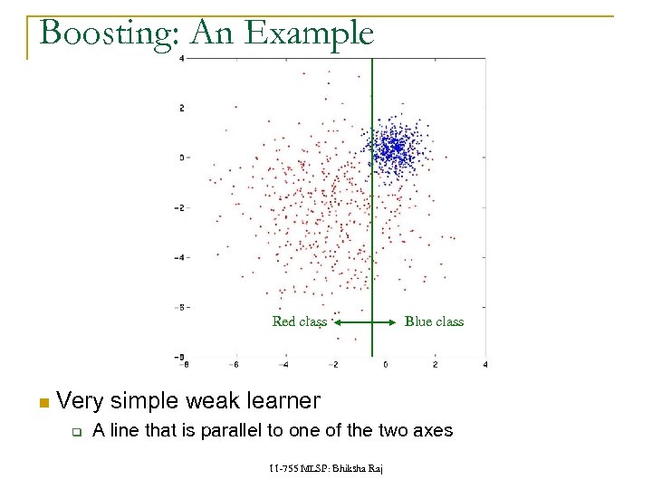Boosting: An Example Red class Blue class Very simple weak learner q A line that is parallel to one of the two axes 11 -755 MLSP: Bhiksha Raj

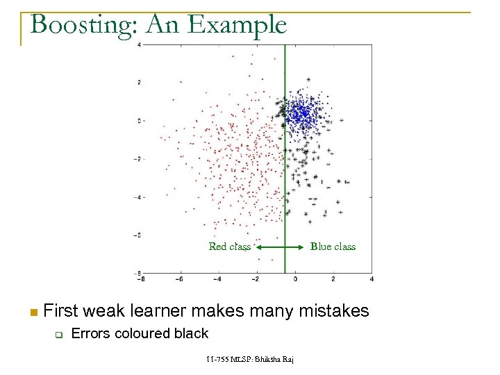Boosting: An Example Red class Blue class First weak learner makes many mistakes q Errors coloured black 11 -755 MLSP: Bhiksha Raj

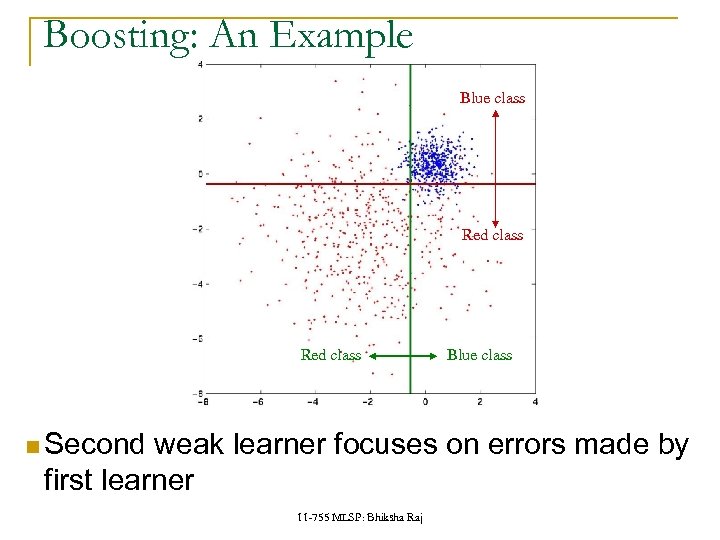Boosting: An Example Blue class Red class Second Blue class weak learner focuses on errors made by first learner 11 -755 MLSP: Bhiksha Raj

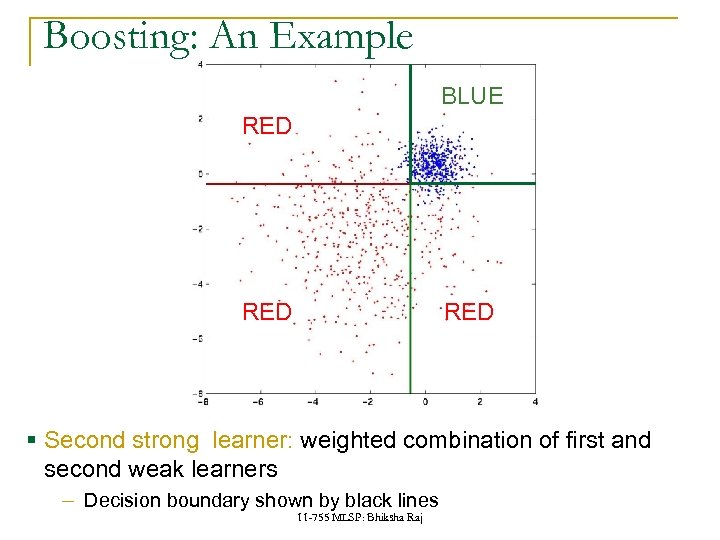Boosting: An Example BLUE RED RED § Second strong learner: weighted combination of first and second weak learners ‒ Decision boundary shown by black lines 11 -755 MLSP: Bhiksha Raj

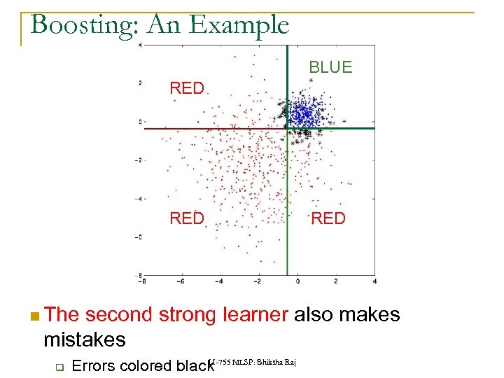Boosting: An Example BLUE RED The RED second strong learner also makes mistakes q 11 -755 Errors colored black MLSP: Bhiksha Raj

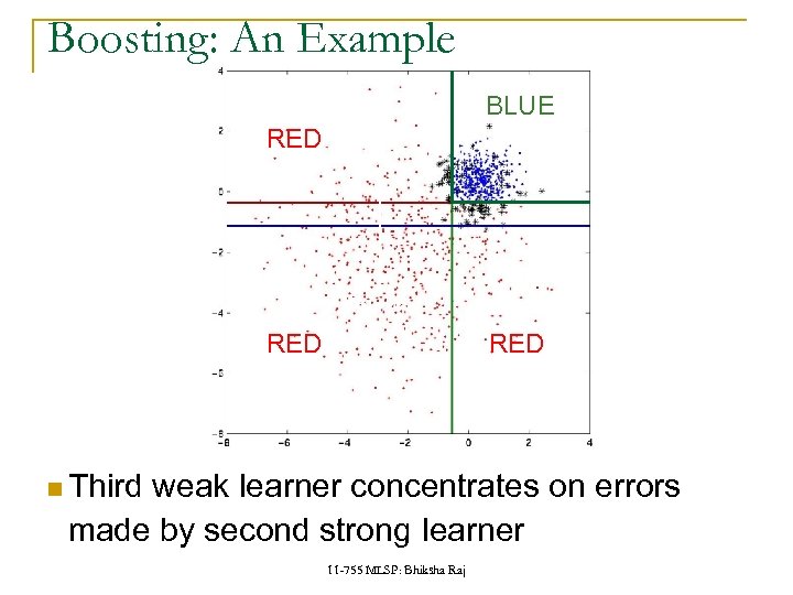Boosting: An Example BLUE RED Blue class Red class RED Third weak learner concentrates on errors made by second strong learner 11 -755 MLSP: Bhiksha Raj

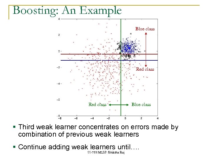Boosting: An Example Blue class Red class Blue class § Third weak learner concentrates on errors made by combination of previous weak learners § Continue adding weak learners until…. 11 -755 MLSP: Bhiksha Raj

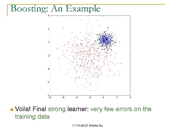Boosting: An Example Voila! Final strong learner: very few errors on the training data 11 -755 MLSP: Bhiksha Raj

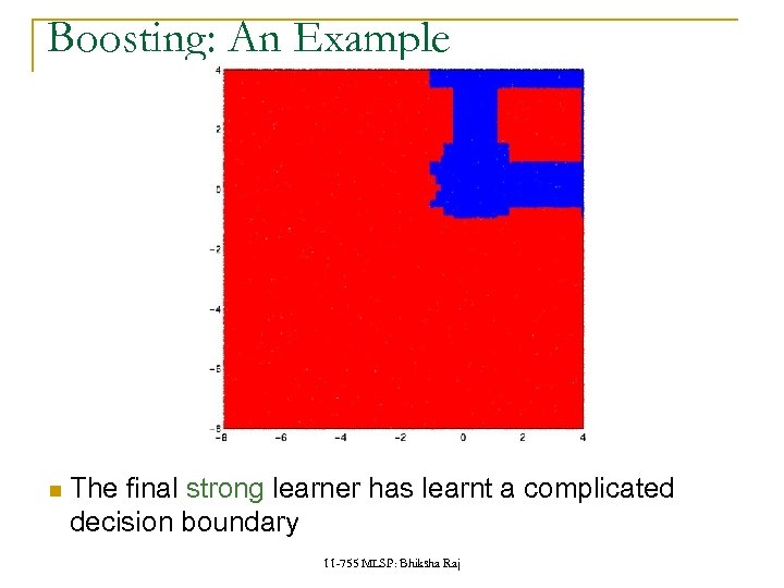Boosting: An Example The final strong learner has learnt a complicated decision boundary 11 -755 MLSP: Bhiksha Raj

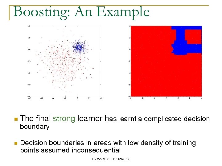Boosting: An Example The final strong learner has learnt a complicated decision boundary Decision boundaries in areas with low density of training points assumed inconsequential 11 -755 MLSP: Bhiksha Raj

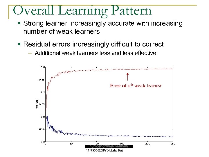Overall Learning Pattern § Strong learner increasingly accurate with increasing number of weak learners § Residual errors increasingly difficult to correct ‒ Additional weak learners less and less effective Error of nth weak learner Error of nth strong learner number of weak learners 11 -755 MLSP: Bhiksha Raj

ADABoost Cannot just add new classifiers that work well only the previously misclassified data Problem: The new classifier will make errors on the points that the earlier classifiers got right q q Not good On test data we have no way of knowing which points were correctly classified by the first classifier Solution: Weight the data when training the second classifier q Use all the data but assign them weights Data that are already correctly classified have less weight Data that are currently incorrectly classified have more weight 11 -755 MLSP: Bhiksha Raj

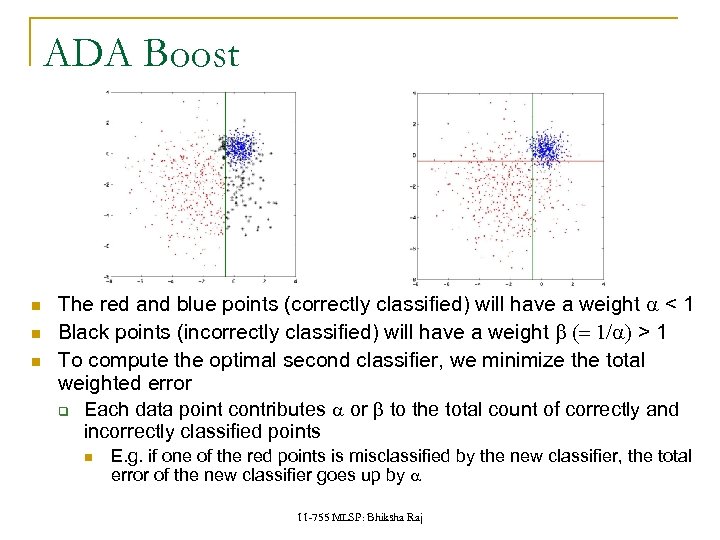ADA Boost The red and blue points (correctly classified) will have a weight a < 1 Black points (incorrectly classified) will have a weight b (= 1/a) > 1 To compute the optimal second classifier, we minimize the total weighted error q Each data point contributes a or b to the total count of correctly and incorrectly classified points E. g. if one of the red points is misclassified by the new classifier, the total error of the new classifier goes up by a 11 -755 MLSP: Bhiksha Raj

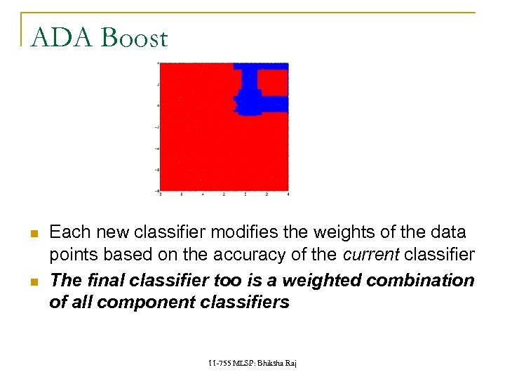ADA Boost Each new classifier modifies the weights of the data points based on the accuracy of the current classifier The final classifier too is a weighted combination of all component classifiers 11 -755 MLSP: Bhiksha Raj

Formalizing the Boosting Concept Given a set of instances (x 1, y 1), (x 2, y 2), … (x. N, y. N) q xi is the set of attributes of the ith instance q y 1 is the class for the ith instance Given a set of classifiers h 1, h 2, … , h. T q hi classifies an instance with attributes x as hi(x) q hi(x) is either -1 or +1 (for a binary classifier) q y 1 can be 1 or -1 (binary classification only) y*h(x) is 1 for all correctly classified points and -1 for incorrectly classified points Devise a function f (h 1(x), h 2(x), …, h. T(x)) such that classification based on f () is superior to classification by any hi(x) q The function is succinctly represented as f (x) 11 -755 MLSP: Bhiksha Raj

The Boosting Concept A simple combiner function: Voting q q q f (x) = Si hi(x) Classifier H(x) = sign(f (x)) = sign(Si hi(x)) Simple majority classifier A simple voting scheme A better combiner function: Boosting q q q f (x) = Si ai hi(x) Can be any real number Classifier H(x) = sign(f (x)) = sign(Si ai hi(x)) A weighted majority classifier The weight ai for any hi(x) is a measure of our trust in hi(x) 11 -755 MLSP: Bhiksha Raj

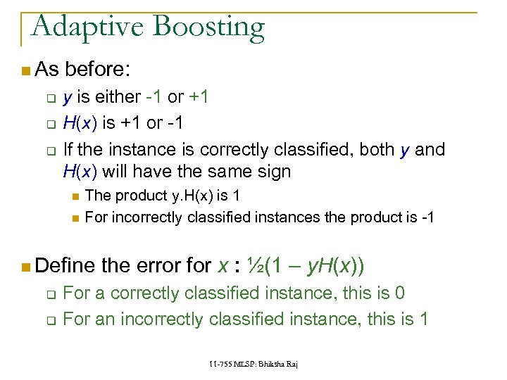Adaptive Boosting As q q q before: y is either -1 or +1 H(x) is +1 or -1 If the instance is correctly classified, both y and H(x) will have the same sign The product y. H(x) is 1 For incorrectly classified instances the product is -1 Define q q the error for x : ½(1 – y. H(x)) For a correctly classified instance, this is 0 For an incorrectly classified instance, this is 1 11 -755 MLSP: Bhiksha Raj

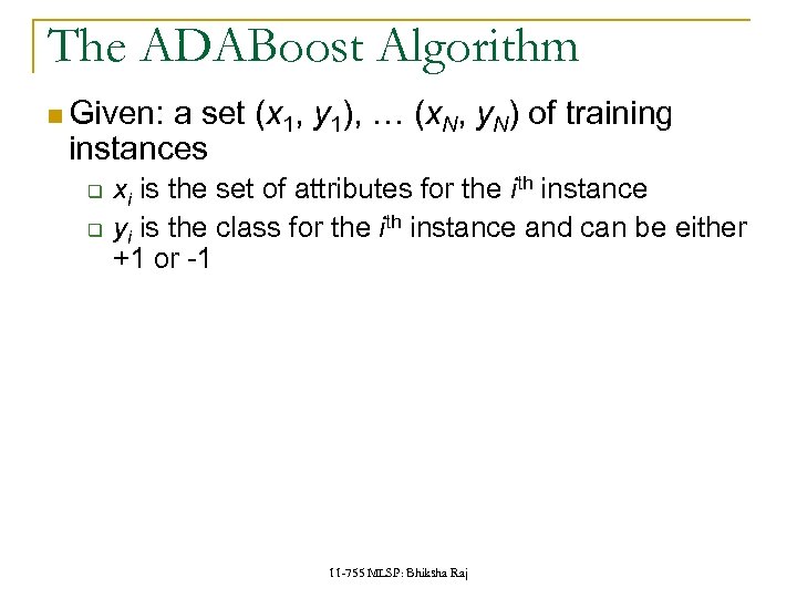The ADABoost Algorithm Given: a set (x 1, y 1), … (x. N, y. N) of training instances q q xi is the set of attributes for the ith instance yi is the class for the ith instance and can be either +1 or -1 11 -755 MLSP: Bhiksha Raj

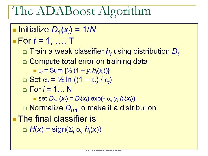The ADABoost Algorithm Initialize D 1(xi) = 1/N For t = 1, …, T q q Train a weak classifier ht using distribution Dt Compute total error on training data q q Set at = ½ ln ((1 – et) / et) For i = 1… N q set Dt+1(xi) = Dt(xi) exp(- at yi ht(xi)) Normalize Dt+1 to make it a distribution The q et = Sum {½ (1 – yi ht(xi))} final classifier is H(x) = sign(St at ht(x)) 11 -755 MLSP: Bhiksha Raj

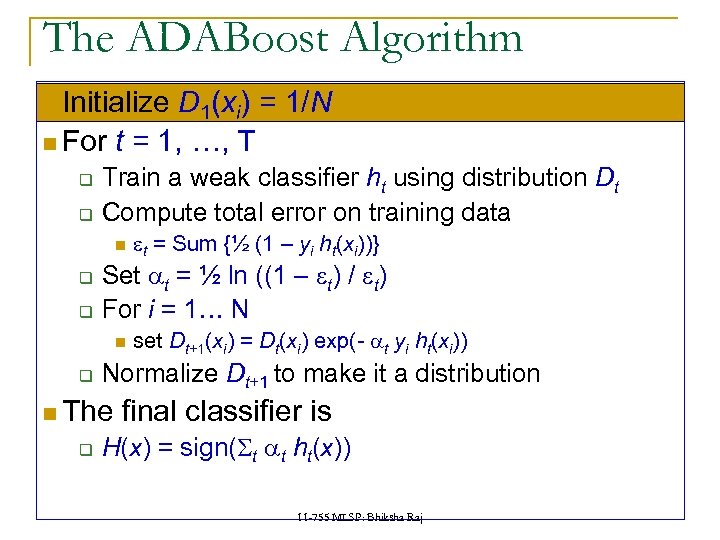The ADABoost Algorithm Initialize D 1(xi) = 1/N For t = 1, …, T q q Train a weak classifier ht using distribution Dt Compute total error on training data q q Set at = ½ ln ((1 – et) / et) For i = 1… N q set Dt+1(xi) = Dt(xi) exp(- at yi ht(xi)) Normalize Dt+1 to make it a distribution The q et = Sum {½ (1 – yi ht(xi))} final classifier is H(x) = sign(St at ht(x)) 11 -755 MLSP: Bhiksha Raj

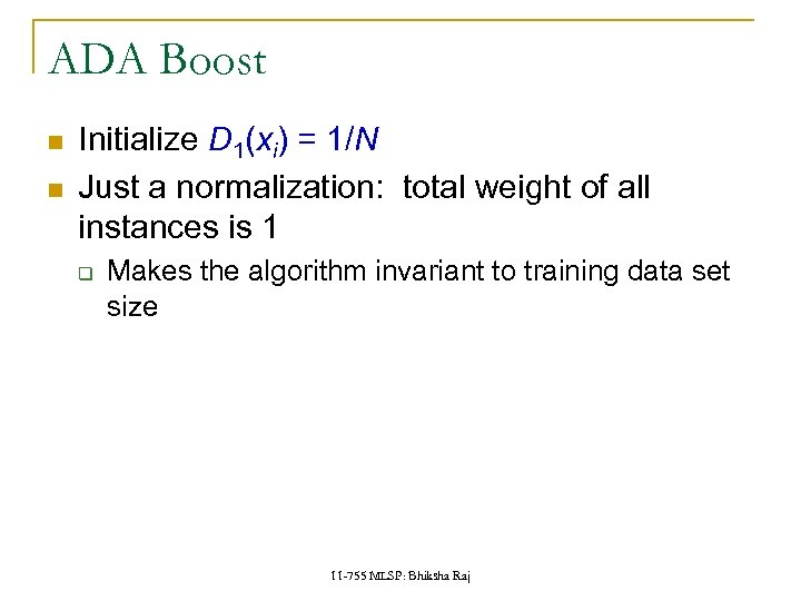ADA Boost Initialize D 1(xi) = 1/N Just a normalization: total weight of all instances is 1 q Makes the algorithm invariant to training data set size 11 -755 MLSP: Bhiksha Raj

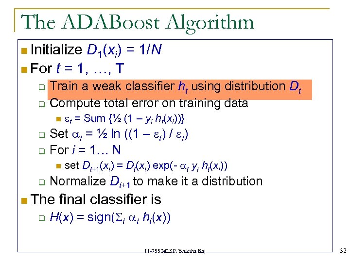The ADABoost Algorithm Initialize D 1(xi) = 1/N For t = 1, …, T q q Train a weak classifier ht using distribution Dt Compute total error on training data q q Set at = ½ ln ((1 – et) / et) For i = 1… N q set Dt+1(xi) = Dt(xi) exp(- at yi ht(xi)) Normalize Dt+1 to make it a distribution The q et = Sum {½ (1 – yi ht(xi))} final classifier is H(x) = sign(St at ht(x)) 11 -755 MLSP: Bhiksha Raj 32

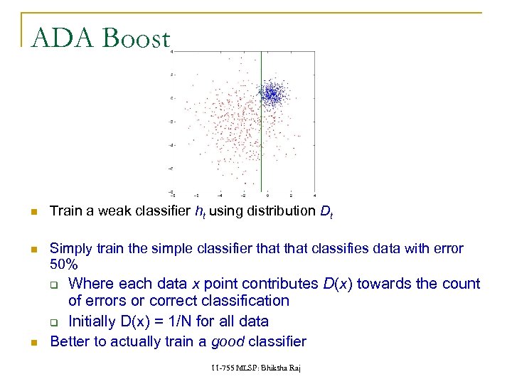ADA Boost Train a weak classifier ht using distribution Dt Simply train the simple classifier that classifies data with error 50% Where each data x point contributes D(x) towards the count of errors or correct classification q Initially D(x) = 1/N for all data Better to actually train a good classifier q 11 -755 MLSP: Bhiksha Raj

The ADABoost Algorithm Initialize D 1(xi) = 1/N For t = 1, …, T q q Train a weak classifier ht using distribution Dt Compute total error on training data q q Set at = ½ ln ((1 – et) / et) For i = 1… N q set Dt+1(xi) = Dt(xi) exp(- at yi ht(xi)) Normalize Dt+1 to make it a distribution The q et = Sum {½ (1 – yi ht(xi))} final classifier is H(x) = sign(St at ht(x)) 11 -755 MLSP: Bhiksha Raj 32

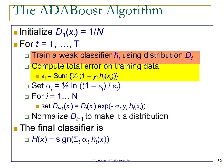
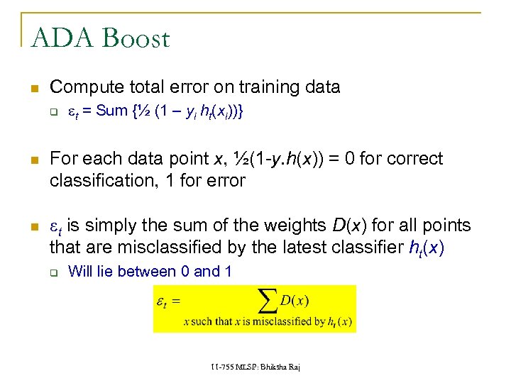ADA Boost Compute total error on training data q et = Sum {½ (1 – yi ht(xi))} For each data point x, ½(1 -y. h(x)) = 0 for correct classification, 1 for error et is simply the sum of the weights D(x) for all points that are misclassified by the latest classifier ht(x) q Will lie between 0 and 1 11 -755 MLSP: Bhiksha Raj

The ADABoost Algorithm Initialize D 1(xi) = 1/N For t = 1, …, T q q Train a weak classifier ht using distribution Dt Compute total error on training data q q Set at = ½ ln ((1 – et) / et) For i = 1… N q set Dt+1(xi) = Dt(xi) exp(- at yi ht(xi)) Normalize Dt+1 to make it a distribution The q et = Sum {½ (1 – yi ht(xi))} final classifier is H(x) = sign(St at ht(x)) 11 -755 MLSP: Bhiksha Raj 32

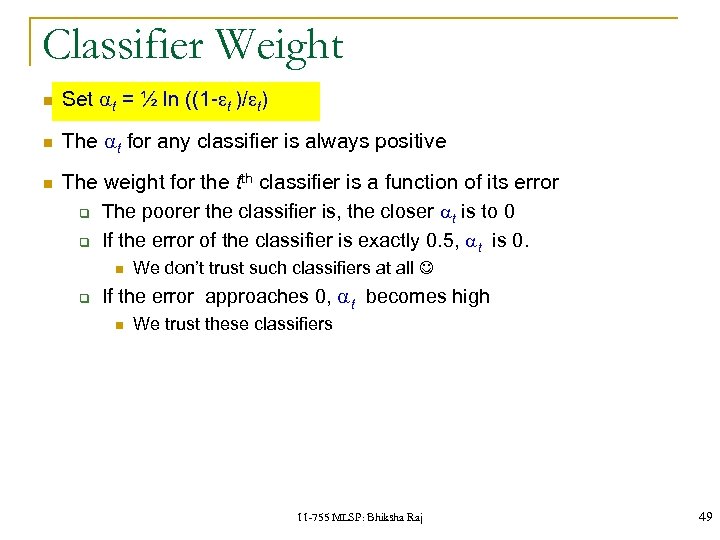Classifier Weight Set at = ½ ln ((1 -et )/et) The at for any classifier is always positive The weight for the tth classifier is a function of its error q The poorer the classifier is, the closer at is to 0 q If the error of the classifier is exactly 0. 5, at is 0. q We don’t trust such classifiers at all If the error approaches 0, at becomes high We trust these classifiers 11 -755 MLSP: Bhiksha Raj 49

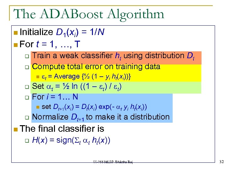The ADABoost Algorithm Initialize D 1(xi) = 1/N For t = 1, …, T q q Train a weak classifier ht using distribution Dt Compute total error on training data q q Set at = ½ ln ((1 – et) / et) For i = 1… N q set Dt+1(xi) = Dt(xi) exp(- at yi ht(xi)) Normalize Dt+1 to make it a distribution The q et = Average {½ (1 – yi ht(xi))} final classifier is H(x) = sign(St at ht(x)) 11 -755 MLSP: Bhiksha Raj 32

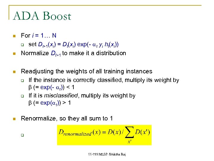ADA Boost For i = 1… N q set Dt+1(xi) = Dt(xi) exp(- at yi ht(xi)) Normalize Dt+1 to make it a distribution Readjusting the weights of all training instances q If the instance is correctly classified, multiply its weight by b (= exp(- at)) < 1 q If it is misclassified, multiply its weight by b (= exp(at)) > 1 Renormalize, so they all sum to 1 q 11 -755 MLSP: Bhiksha Raj

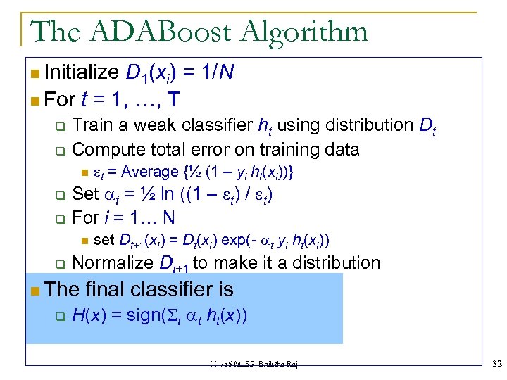The ADABoost Algorithm Initialize D 1(xi) = 1/N For t = 1, …, T q q Train a weak classifier ht using distribution Dt Compute total error on training data q q Set at = ½ ln ((1 – et) / et) For i = 1… N q set Dt+1(xi) = Dt(xi) exp(- at yi ht(xi)) Normalize Dt+1 to make it a distribution The q et = Average {½ (1 – yi ht(xi))} final classifier is H(x) = sign(St at ht(x)) 11 -755 MLSP: Bhiksha Raj 32

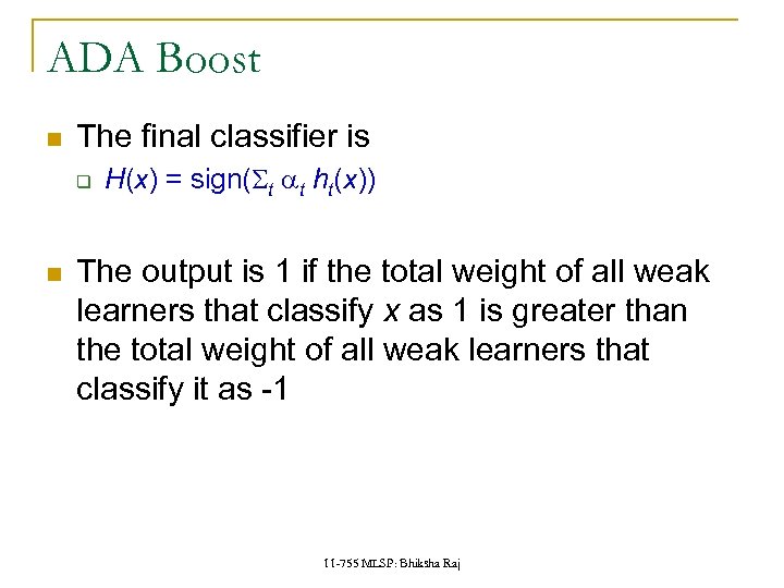ADA Boost The final classifier is q H(x) = sign(St at ht(x)) The output is 1 if the total weight of all weak learners that classify x as 1 is greater than the total weight of all weak learners that classify it as -1 11 -755 MLSP: Bhiksha Raj

Next Class Fernando De La Torre We will continue with Viola Jones after a few classes 11 -755 MLSP: Bhiksha Raj

Boosting and Face Detection Boosting forms the basis of the most common technique for face detection today: The Viola -Jones algorithm. 11 -755 MLSP: Bhiksha Raj

The problem of face detection 1. Defining Features q Should we be searching for noses, eyebrows etc. ? q Or something simpler 2. Selecting Features q Nice, but expensive Of all the possible features we can think of, which ones make sense 3. Classification: Combining evidence q How does one combine the evidence from the different features? 11 -755 MLSP: Bhiksha Raj

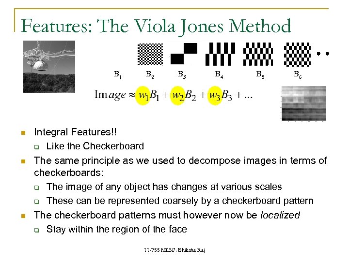Features: The Viola Jones Method B 1 B 2 B 3 B 4 B 5 B 6 Integral Features!! q Like the Checkerboard The same principle as we used to decompose images in terms of checkerboards: q The image of any object has changes at various scales q These can be represented coarsely by a checkerboard pattern The checkerboard patterns must however now be localized q Stay within the region of the face 11 -755 MLSP: Bhiksha Raj

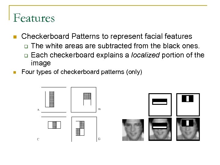Features Checkerboard Patterns to represent facial features q The white areas are subtracted from the black ones. q Each checkerboard explains a localized portion of the image Four types of checkerboard patterns (only)

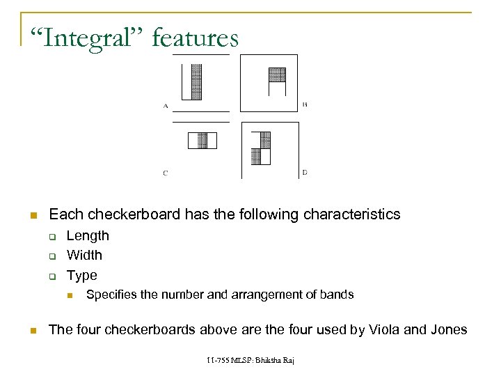“Integral” features Each checkerboard has the following characteristics q q q Length Width Type Specifies the number and arrangement of bands The four checkerboards above are the four used by Viola and Jones 11 -755 MLSP: Bhiksha Raj

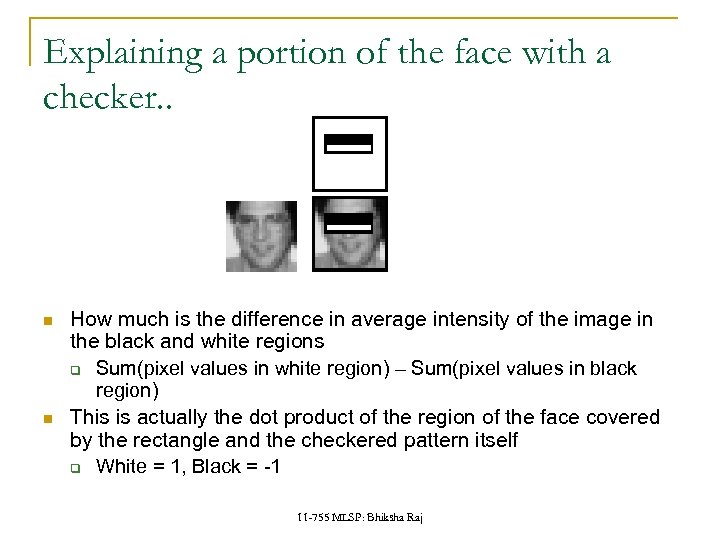Explaining a portion of the face with a checker. . How much is the difference in average intensity of the image in the black and white regions q Sum(pixel values in white region) – Sum(pixel values in black region) This is actually the dot product of the region of the face covered by the rectangle and the checkered pattern itself q White = 1, Black = -1 11 -755 MLSP: Bhiksha Raj

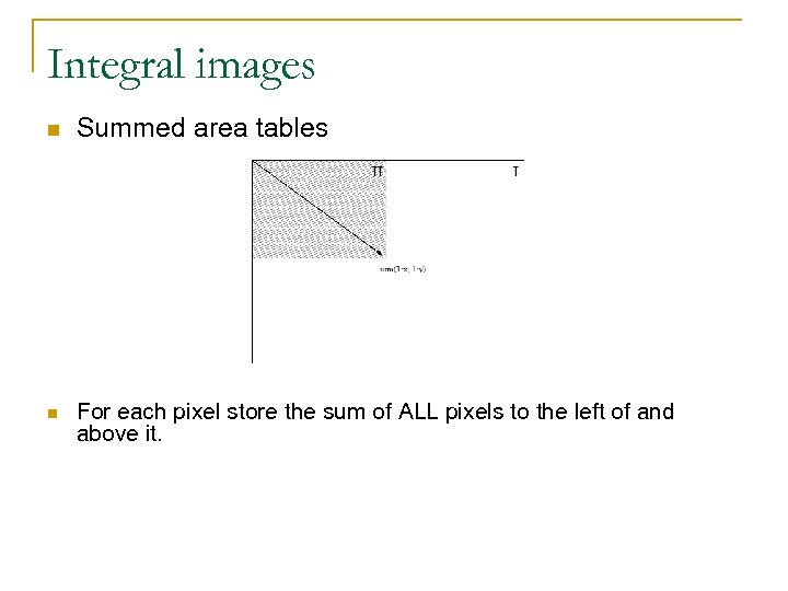Integral images Summed area tables For each pixel store the sum of ALL pixels to the left of and above it.

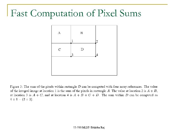Fast Computation of Pixel Sums 11 -755 MLSP: Bhiksha Raj

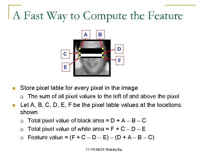A Fast Way to Compute the Feature A C B D F E Store pixel table for every pixel in the image q The sum of all pixel values to the left of and above the pixel Let A, B, C, D, E, F be the pixel table values at the locations shown q Total pixel value of black area = D + A – B – C q Total pixel value of white area = F + C – D – E q Feature value = (F + C – D – E) – (D + A – B – C) 11 -755 MLSP: Bhiksha Raj

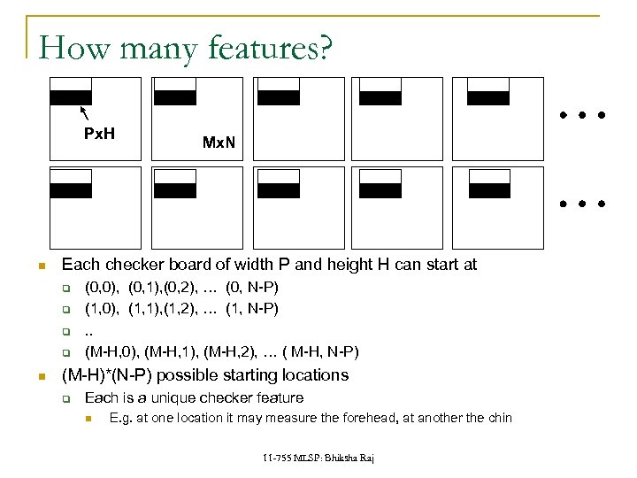How many features? Px. H Each checker board of width P and height H can start at q q Mx. N (0, 0), (0, 1), (0, 2), … (0, N-P) (1, 0), (1, 1), (1, 2), … (1, N-P). . (M-H, 0), (M-H, 1), (M-H, 2), … ( M-H, N-P) (M-H)*(N-P) possible starting locations q Each is a unique checker feature E. g. at one location it may measure the forehead, at another the chin 11 -755 MLSP: Bhiksha Raj

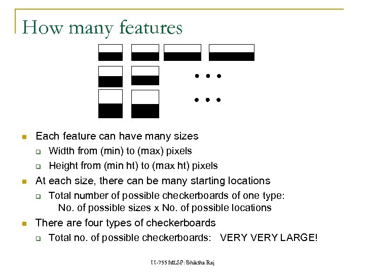How many features Each feature can have many sizes q Width from (min) to (max) pixels q Height from (min ht) to (max ht) pixels At each size, there can be many starting locations q Total number of possible checkerboards of one type: No. of possible sizes x No. of possible locations There are four types of checkerboards q Total no. of possible checkerboards: VERY LARGE! 11 -755 MLSP: Bhiksha Raj

Learning: No. of features Analysis performed on images of 24 x 24 pixels only q Reduces the no. of possible features to about 180000 Restrict checkerboard size q q Minimum of 8 pixels wide Minimum of 8 pixels high q Other limits, e. g. 4 pixels may be used too Reduces no. of checkerboards to about 50000 11 -755 MLSP: Bhiksha Raj

No. of features Each possible checkerboard gives us one feature A total of up to 180000 features derived from a 24 x 24 image! Every 24 x 24 image is now represented by a set of 180000 numbers q This is the set of features we will use for classifying if it is a face or not! 11 -755 MLSP: Bhiksha Raj

The Classifier The Viola-Jones algorithm uses a simple Boosting based classifier Each “weak learner” is a simple threshold At each stage find the best feature to classify the data with q I. e the feature that gives us the best classification of all the training data q Training data includes many examples of faces and non-face images The classification rule is of the kind If feature > threshold, face (or if feature < threshold, face) The optimal value of “threshold” must also be determined. 11 -755 MLSP: Bhiksha Raj

The Weak Learner Training (for each weak learner): q For each feature f (of all 180000 features) Find a threshold q(f) and polarity p(f) (p(f) = -1 or p(f) = 1) such that (f > p(f)*q(f)) performs the best classification of faces q q q Lowest overall error in classifying all training data § Error counted over weighted samples Let the optimal overall error f be error(f) Find the feature f’ such that error(f’) is lowest The weak learner is the test (f’ > p(f’)*q(f’)) => face Note that the procedure for learning weak learners also identifies the most useful features for face recognition 11 -755 MLSP: Bhiksha Raj

The Viola Jones Classifier A boosted threshold-based classifier First weak learner: Find the best feature, and its optimal threshold q Second weak learner: Find the best feature, for the weighted training data, and its threshold (weighting from one weak learner) Third weak learner: Find the best feature for the weighted data and its optimal threshold (weighting from two weak learners) q Fourth weak learner: Find the best feature for the weighted data and its optimal threhsold (weighting from three weak learners) §. . 11 -755 MLSP: Bhiksha Raj

To Train Collect a large number of histogram equalized facial images q q Collect a much larger set of 24 x 24 non-face images of all kinds q q Resize all of them to 24 x 24 These are our “face” training set Each of them is histogram equalized These are our “non-face” training set Train a boosted classifier 11 -755 MLSP: Bhiksha Raj

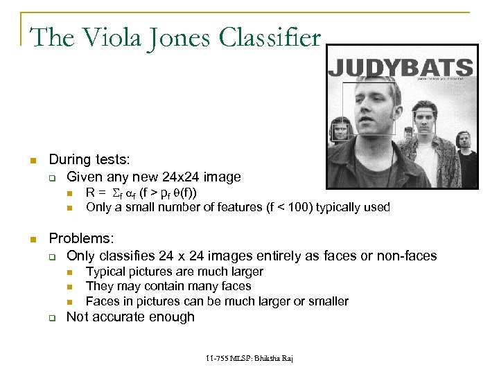The Viola Jones Classifier During tests: q Given any new 24 x 24 image R = Sf af (f > pf q(f)) Only a small number of features (f < 100) typically used Problems: q Only classifies 24 x 24 images entirely as faces or non-faces q Typical pictures are much larger They may contain many faces Faces in pictures can be much larger or smaller Not accurate enough 11 -755 MLSP: Bhiksha Raj

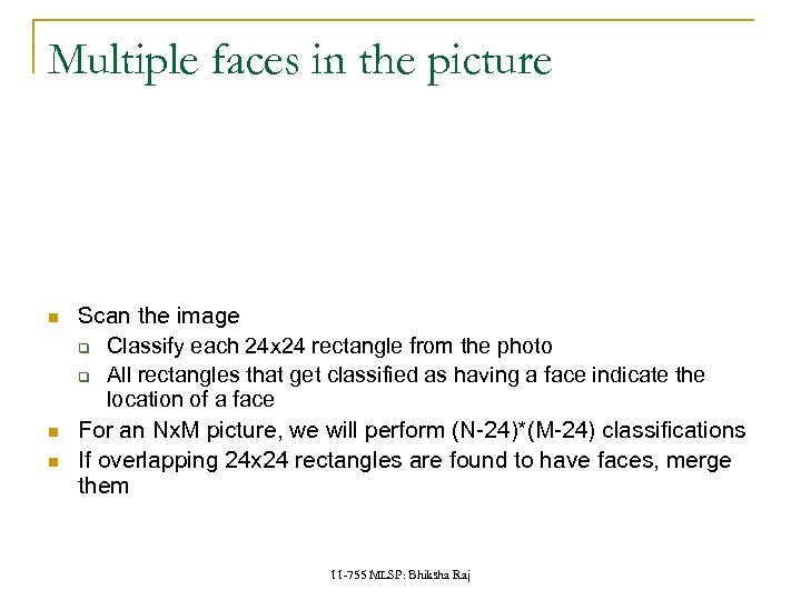Multiple faces in the picture Scan the image q Classify each 24 x 24 rectangle from the photo q All rectangles that get classified as having a face indicate the location of a face For an Nx. M picture, we will perform (N-24)*(M-24) classifications If overlapping 24 x 24 rectangles are found to have faces, merge them 11 -755 MLSP: Bhiksha Raj

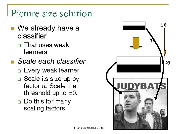Picture size solution We already have a classifier q That uses weak learners Scale each classifier q q q Every weak learner Scale its size up by factor a. Scale threshold up to aq. Do this for many scaling factors 11 -755 MLSP: Bhiksha Raj f, q 2 x f, 2 q

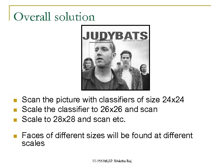Overall solution Scan the picture with classifiers of size 24 x 24 Scale the classifier to 26 x 26 and scan Scale to 28 x 28 and scan etc. Faces of different sizes will be found at different scales 11 -755 MLSP: Bhiksha Raj

False Rejection vs. False detection False Rejection: There’s a face in the image, but the classifier misses it q Rejects the hypothesis that there’s a face False detection: Recognizes a face when there is none. Classifier: q Standard boosted classifier: H(x) = sign(St at ht(x)) q Modified classifier H(x) = sign(St at ht(x) + Y) St at ht(x) is a measure of certainty q q The higher it is, the more certain we are that we found a face If Y is large, then we assume the presence of a face even when we are not sure By increasing Y, we can reduce false rejection, while increasing false detection 11 -755 MLSP: Bhiksha Raj

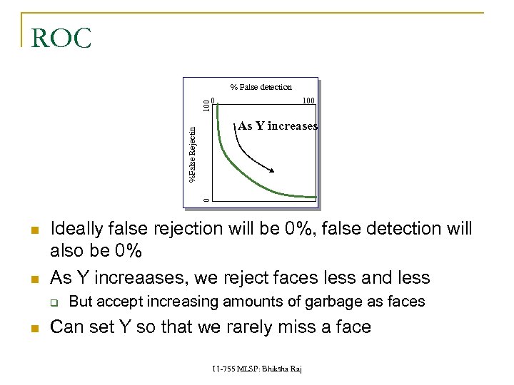ROC % False detection 100 0 vsfalseneg determined by 0 %False Rejectin As Y increases Ideally false rejection will be 0%, false detection will also be 0% As Y increaases, we reject faces less and less q But accept increasing amounts of garbage as faces Can set Y so that we rarely miss a face 11 -755 MLSP: Bhiksha Raj

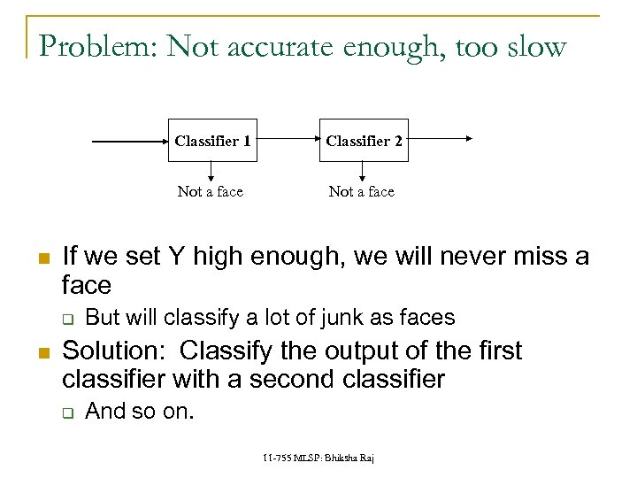Problem: Not accurate enough, too slow Classifier 1 Not a face If we set Y high enough, we will never miss a face q Classifier 2 But will classify a lot of junk as faces Solution: Classify the output of the first classifier with a second classifier q And so on. 11 -755 MLSP: Bhiksha Raj

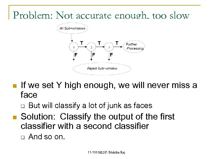Problem: Not accurate enough, too slow If we set Y high enough, we will never miss a face q But will classify a lot of junk as faces Solution: Classify the output of the first classifier with a second classifier q And so on. 11 -755 MLSP: Bhiksha Raj

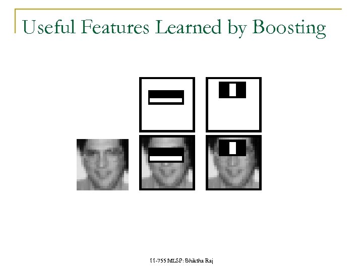Useful Features Learned by Boosting 11 -755 MLSP: Bhiksha Raj

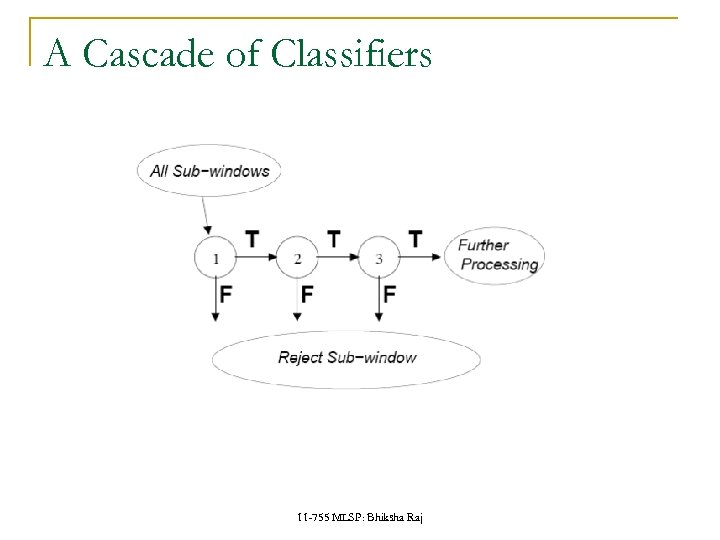A Cascade of Classifiers 11 -755 MLSP: Bhiksha Raj

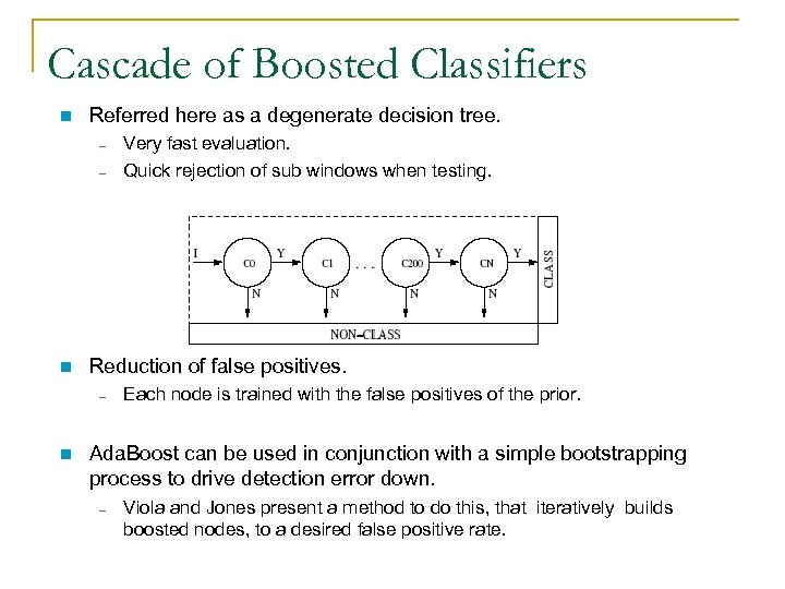Cascade of Boosted Classifiers Referred here as a degenerate decision tree. – – Reduction of false positives. – Very fast evaluation. Quick rejection of sub windows when testing. Each node is trained with the false positives of the prior. Ada. Boost can be used in conjunction with a simple bootstrapping process to drive detection error down. – Viola and Jones present a method to do this, that iteratively builds boosted nodes, to a desired false positive rate.

Detection in Real Images Basic classifier operates on 24 x 24 subwindows Scaling: q Scale the detector (rather than the images) q Features can easily be evaluated at any scale q Scale by factors of 1. 25 Location: q Move detector around the image (e. g. , 1 pixel increments) Final Detections q A real face may result in multiple nearby detections q Postprocess detected subwindows to combine overlapping detections into a single detection 11 -755 MLSP: Bhiksha Raj

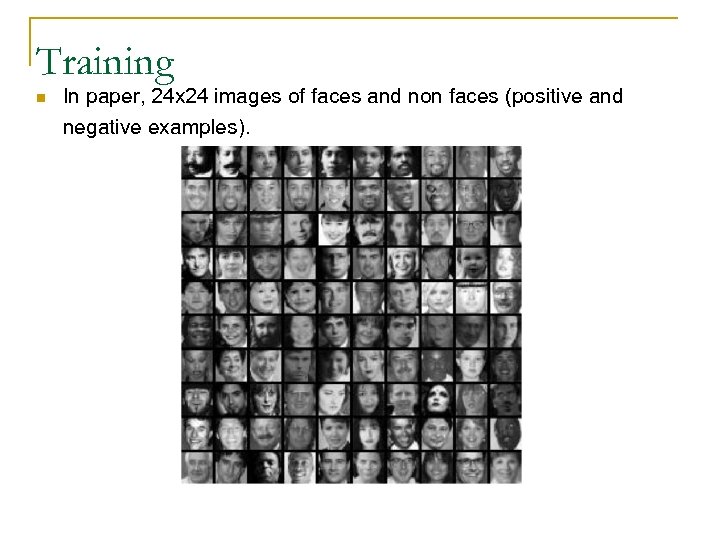Training In paper, 24 x 24 images of faces and non faces (positive and negative examples).

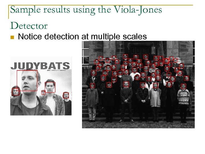Sample results using the Viola-Jones Detector Notice detection at multiple scales

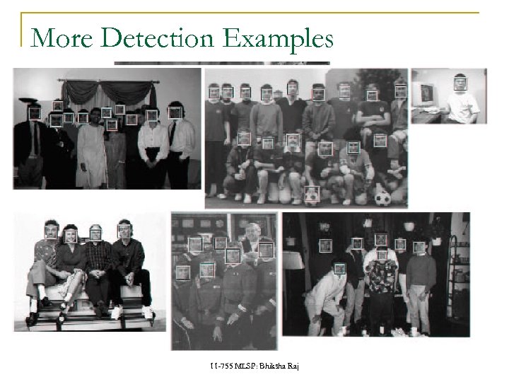More Detection Examples 11 -755 MLSP: Bhiksha Raj

Practical implementation Details discussed in Viola-Jones paper Training time = weeks (with 5 k faces and 9. 5 k nonfaces) Final detector has 38 layers in the cascade, 6060 features 700 Mhz processor: q Can process a 384 x 288 image in 0. 067 seconds (in 2003 when paper was written) 11 -755 MLSP: Bhiksha Raj