11 16 Learning Improving the performance of the

11/16

Learning Improving the performance of the agent -w. r. t. the external performance measure Dimensions: What can be learned? --Any of the boxes representing the agent’s knowledge --action description, effect probabilities, causal relations in the world (and the probabilities of causation), utility models (sort of through credit assignment), sensor data interpretation models What feedback is available? --Supervised, unsupervised, “reinforcement” learning --Credit assignment problem What prior knowledge is available? -- “Tabularasa” (agent’s head is a blank slate) or pre-existing knowledge

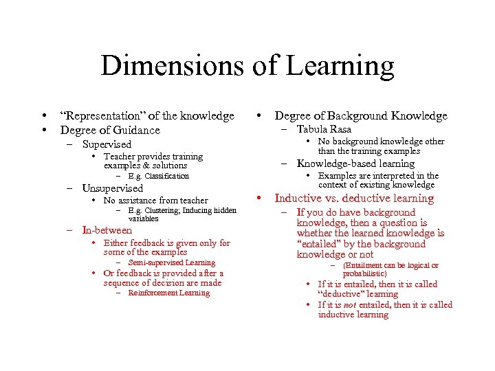Dimensions of Learning • • “Representation” of the knowledge Degree of Guidance • – Tabula Rasa • No background knowledge other than the training examples – Supervised • Teacher provides training examples & solutions – Knowledge-based learning • Examples are interpreted in the context of existing knowledge – E. g. Classification – Unsupervised • No assistance from teacher – E. g. Clustering; Inducing hidden variables – In-between • Either feedback is given only for some of the examples – Semi-supervised Learning • Or feedback is provided after a sequence of decision are made – Reinforcement Learning Degree of Background Knowledge • Inductive vs. deductive learning – If you do have background knowledge, then a question is whether the learned knowledge is “entailed” by the background knowledge or not – (Entailment can be logical or probabilistic) • If it is entailed, then it is called “deductive” learning • If it is not entailed, then it is called inductive learning

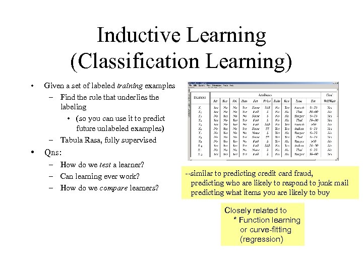Inductive Learning (Classification Learning) • Given a set of labeled training examples – Find the rule that underlies the labeling • (so you can use it to predict future unlabeled examples) – Tabula Rasa, fully supervised • Qns: – How do we test a learner? – Can learning ever work? – How do we compare learners? --similar to predicting credit card fraud, predicting who are likely to respond to junk mail predicting what items you are likely to buy Closely related to * Function learning or curve-fitting (regression)

K-Nearest Neighbor • An unseen instance’s class is determined by its nearest neighbor – Or the majority label of its nearest k neighbors • Real Issue: Getting the right distance metric to decide who are the neighbors… • One of the most obvious classification algorithms – Skips the middle stage and lets the examples be their own pattern • A variation is to “cluster” the training examples and remember the prototypes for each cluster (reduces the number of things remembered)

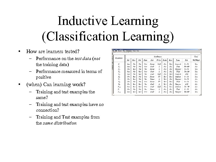Inductive Learning (Classification Learning) • How are learners tested? – Performance on the test data (not the training data) – Performance measured in terms of positive • (when) Can learning work? – Training and test examples the same? – Training and test examples have no connection? – Training and Test examples from the same distribution

A good hypothesis will have fewest false positives (Fh+) and fewest false negatives (Fh-) [Ideally, we want them to be zero] False +ve: The learner classifies the example as +ve, but it is actually -ve Rank(h) = f(Fh+, Fh-) --f depends on the domain by default f=Sum; but can give different weights to different errors (Cost-based learning) Medical domain --Higher cost for F--But also high cost for F+ Spam Mailer --Very low cost for F+ --higher cost for FTerrorist/Criminal Identification --High cost for F+ (for the individual) --High cost for F- (for the society) Ranking hypotheses H 1: Russell waits only in italian restaurants false +ves: X 10, false –ves: X 1, X 3, X 4, X 8, X 12 H 2: Russell waits only in cheap french restaurants False +ves: False –ves: X 1, X 3, X 4, X 6, X 8, X 12

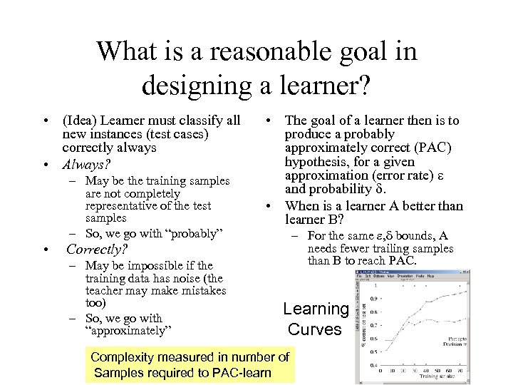What is a reasonable goal in designing a learner? • (Idea) Learner must classify all new instances (test cases) correctly always • Always? – May be the training samples are not completely representative of the test samples – So, we go with “probably” • • The goal of a learner then is to produce a probably approximately correct (PAC) hypothesis, for a given approximation (error rate) e and probability d. • When is a learner A better than learner B? – For the same e, d bounds, A needs fewer trailing samples than B to reach PAC. Correctly? – May be impossible if the training data has noise (the teacher may make mistakes too) – So, we go with “approximately” Learning Curves Complexity measured in number of Samples required to PAC-learn

Inductive Learning (Classification Learning) • Given a set of labeled examples, and a space of hypotheses – Find the rule that underlies the labeling • (so you can use it to predict future unlabeled examples) – Tabularasa, fully supervised • Idea: – Loop through all hypotheses • Rank each hypothesis in terms of its match to data • Pick the best hypothesis • • – Main variations: Bias: the “sort” of rule are you looking for? – If you are looking for only conjunctive hypotheses, there are just 3 n Search: – Greedy search – Decision tree learner – Systematic search – Version space learner – Iterative search – Neural net learner It can be shown that sample complexity of PAC learning is proportional to 1/e, 1/d AND log |H| The main problem is that the space of hypotheses is too large Given examples described in terms of n boolean variables n There are 2 2 different hypotheses For 6 features, there are 18, 446, 744, 073, 709, 551, 616 hypotheses

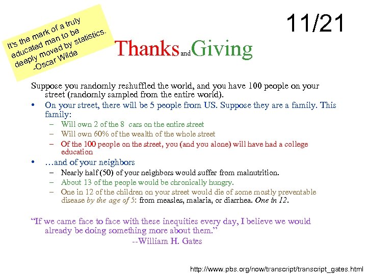uly a tr of ark n to be tistics. m the d ma by sta It's ate c ved edu ly mo Wilde p r dee -Osca Thanks Giving 11/21 and Suppose you randomly reshuffled the world, and you have 100 people on your street (randomly sampled from the entire world). • On your street, there will be 5 people from US. Suppose they are a family. This family: – Will own 2 of the 8 cars on the entire street – Will own 60% of the wealth of the whole street – Of the 100 people on the street, you (and you alone) will have had a college education • …and of your neighbors – Nearly half (50) of your neighbors would suffer from malnutrition. – About 13 of the people would be chronically hungry. – One in 12 of the children on your street would die of some mostly preventable disease by the age of 5: from measles, malaria, or diarrhea. One in 12. “If we came face to face with these inequities every day, I believe we would already be doing something more about them. ” --William H. Gates http: //www. pbs. org/now/transcript_gates. html

Administrative • Homework 4 is gathering mass… – (insert ominous sound effects here) • Project 4 will be the last coding project – You can submit until tomorrow (make-up class) without penalty; and with 3 p% penalty until Monday • Make-up class tomorrow BYENG 210 – Note: This is the second floor of Brickyard bldg (near the instructional labs; and on the same floor as advising office)

We defined inductive learning problem… • So, let’s get started learning already. .

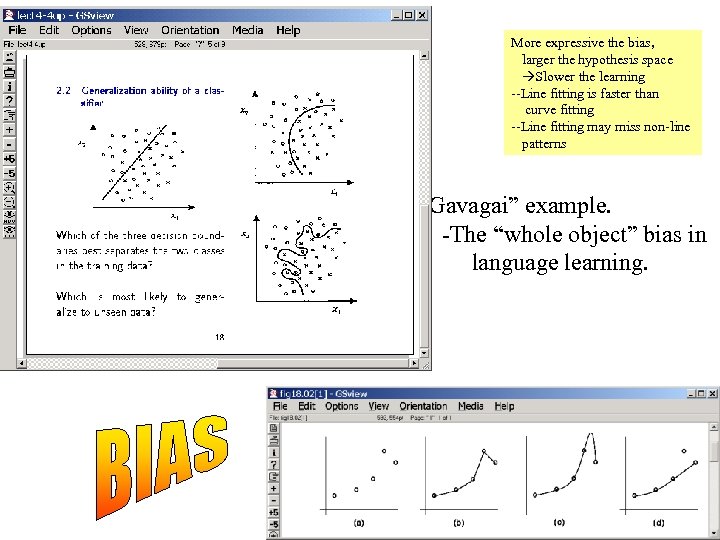More expressive the bias, larger the hypothesis space Slower the learning --Line fitting is faster than curve fitting --Line fitting may miss non-line patterns “Gavagai” example. -The “whole object” bias in language learning.

Uses different biases in predicting Russel’s waiting habbits If patrons=full and day=Friday then wait (0. 3/0. 7) If wait>60 and Reservation=no then wait (0. 4/0. 9) K-nearest neighbors Decision Trees --Examples are used to --Learn topology --Order of questions Association rules --Examples are used to --Learn support and confidence of association rules SVMs Neural Nets --Examples are used to --Learn topology --Learn edge weights Naïve bayes (bayesnet learning) --Examples are used to --Learn topology --Learn CPTs

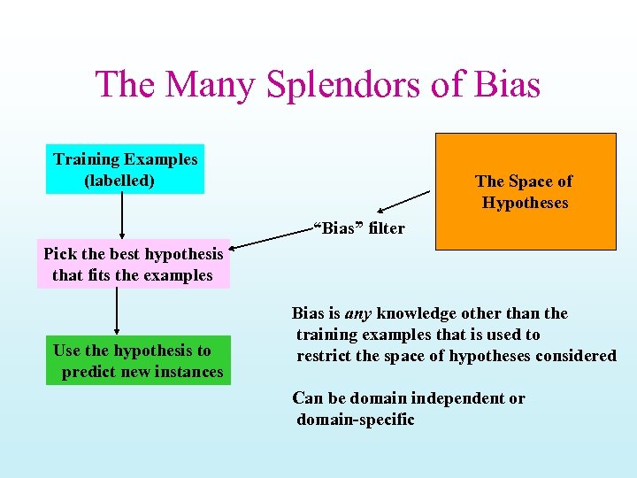The Many Splendors of Bias Training Examples (labelled) The Space of Hypotheses “Bias” filter Pick the best hypothesis that fits the examples Use the hypothesis to predict new instances Bias is any knowledge other than the training examples that is used to restrict the space of hypotheses considered Can be domain independent or domain-specific

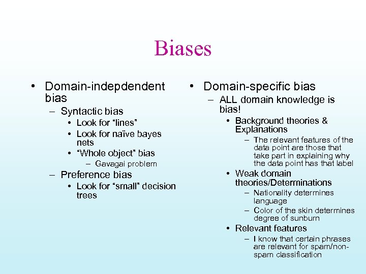Biases • Domain-indepdendent bias – Syntactic bias • Look for “lines” • Look for naïve bayes nets • “Whole object” bias – Gavagai problem – Preference bias • Look for “small” decision trees • Domain-specific bias – ALL domain knowledge is bias! • Background theories & Explanations – The relevant features of the data point are those that take part in explaining why the data point has that label • Weak domain theories/Determinations – Nationality determines language – Color of the skin determines degree of sunburn • Relevant features – I know that certain phrases are relevant for spam/nonspam classification

Bias & Learning cost • Strong Bias smaller filtered hypothesis space – Lower learning cost! (because you need fewer examples to rank the hypotheses!) • Suppose I have decided that hair length determines pass/fail grade in the class, then I can “learn” the concept with a _single_ example! – Cuts down the concepts you can learn accurately • Strong Bias fewer parameters for describing the hypthesis – Lower learning cost!! – For discrete variable learning cases, the sample complexity can be shown to be proportional to log(|H|) where H is the hypothesis space

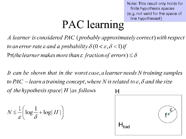PAC learning Note: This result only holds for finite hypothesis spaces (e. g. not valid for the space of line hypotheses!)

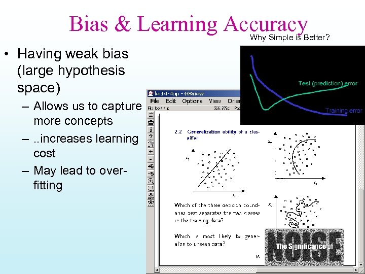Bias & Learning Accuracy Why Simple is Better? • Having weak bias (large hypothesis space) – Allows us to capture more concepts –. . increases learning cost – May lead to overfitting

Tastes Great/Less Filling • Biases are essential for survival of an agent! – You must need biases to just make learning tractable • “Whole object bias” used by kids in language acquisition • Biases put blinders on the learner—filtering away (possibly more accurate) hypotheses – “God doesn’t play dice with the universe” (Einstein) – “Color of Skin relevant to predicting crime” (Billy Bennett—Former Education Secretary)

Those who ignore easily available domain knowledge are doomed to re-learn it… Santayana’s brother Domain-knowledge & Learning • Classification learning is a problem addressed by both people from AI (machine learning) and Statistics • Statistics folks tend to “distrust” domain-specific bias. – Let the data speak for itself… –. . but this is often futile. The very act of “describing” the data points introduces bias (in terms of the features you decided to use to describe them. . ) • …but much human learning occurs because of strong domainspecific bias. . • Machine learning is torn by these competing influences. . – In most current state of the art algorithms, domain knowledge is allowed to influence learning only through relatively narrow avenues/formats (E. g. through “kernels”) • Okay in domains where there is very little (if any) prior knowledge (e. g. what part of proteins are doing what cellular function) • . . restrictive in domains where there already exists human expertise. .

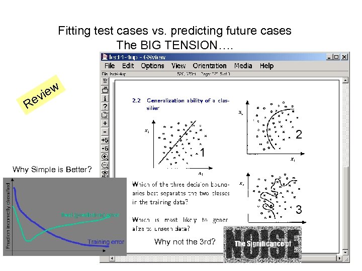Fitting test cases vs. predicting future cases The BIG TENSION…. iew ev R 2 1 Why Simple is Better? 3 Why not the 3 rd?

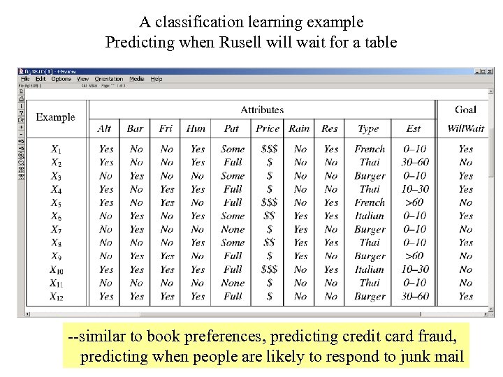A classification learning example Predicting when Rusell will wait for a table --similar to book preferences, predicting credit card fraud, predicting when people are likely to respond to junk mail

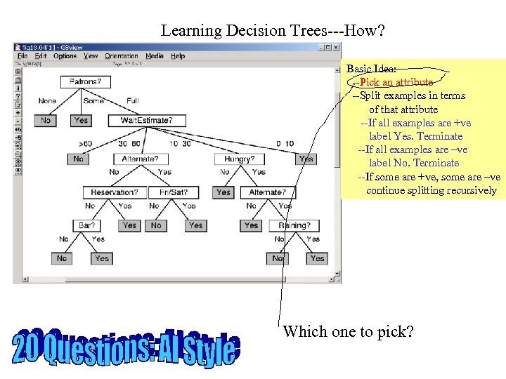Learning Decision Trees---How? Basic Idea: --Pick an attribute --Split examples in terms of that attribute --If all examples are +ve label Yes. Terminate --If all examples are –ve label No. Terminate --If some are +ve, some are –ve continue splitting recursively Which one to pick?

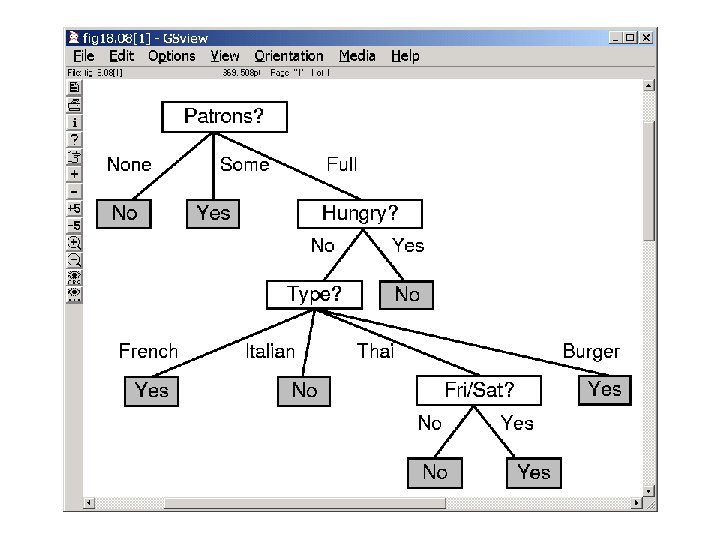
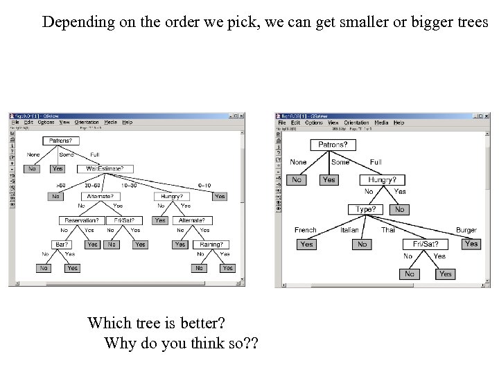Depending on the order we pick, we can get smaller or bigger trees Which tree is better? Why do you think so? ?

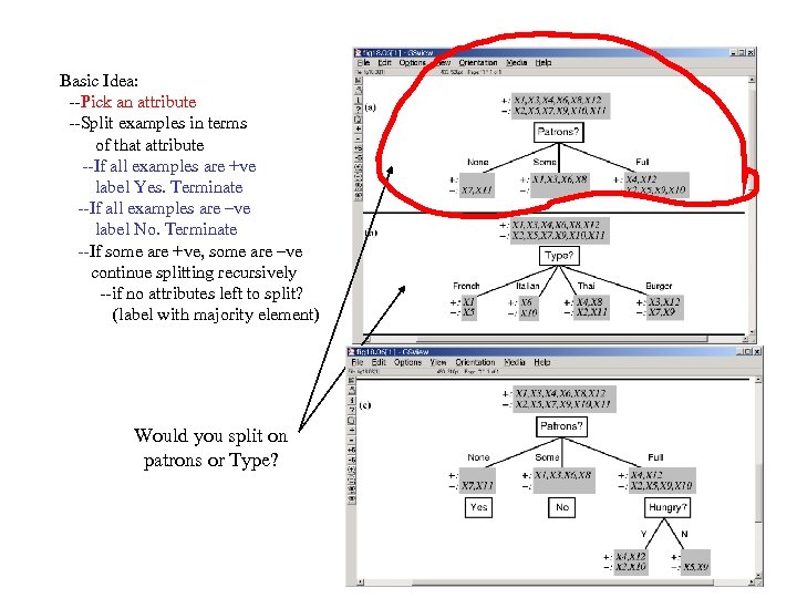Basic Idea: --Pick an attribute --Split examples in terms of that attribute --If all examples are +ve label Yes. Terminate --If all examples are –ve label No. Terminate --If some are +ve, some are –ve continue splitting recursively --if no attributes left to split? (label with majority element) Would you split on patrons or Type?

The Information Gain Computation P+ : N+ /(N++N-) P- : N- /(N++N-) # expected comparisons needed to tell whether a given example is +ve or -ve I(P+ , , P-) = -P+ log(P+) - P- log(P- ) N+ NThe difference is the information gain Splitting on feature fk N 1 + N 1 - I(P 1+ , , P 1 -) N 2 + N 2 - I(P 2+ , , P 2 -) Nk + Nk - I(Pk+ , , Pk-) So, pick the feature with the largest Info Gain I. e. smallest residual info k Given k mutually exclusive and exhaustive events E 1…. Ek whose probabilities are p 1…. pk The “information” content (entropy) is defined as S i -pi log 2 pi A split is good if it reduces the entropy. . S i=1 [Ni+ + Ni- ]/[N+ + N-] I(Pi+ , , Pi-)

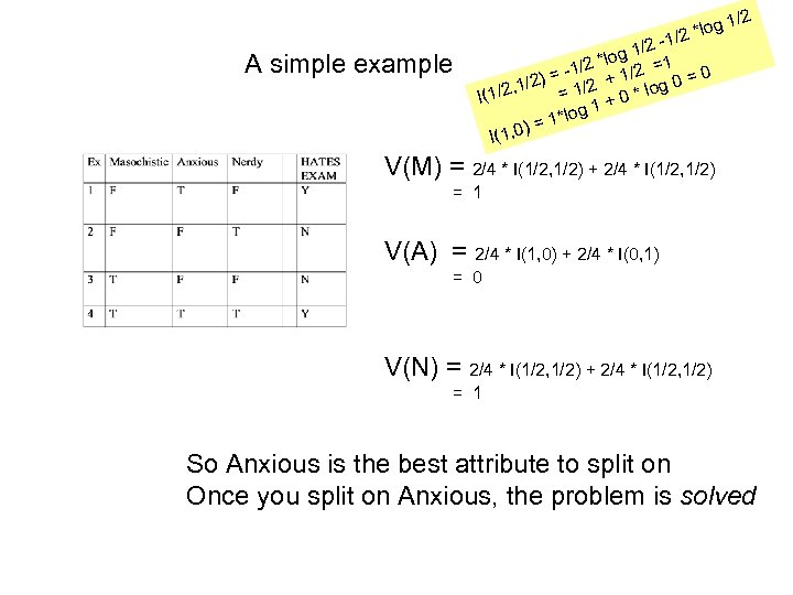A simple example *log -1/2 /2 log 1 =1 /2 * /2 0 = -1 1 1/2) 2 + * log 0 = , = 1/ + 0 I(1/2 g 1 1*lo )= I(1, 0 1/2 V(M) = 2/4 * I(1/2, 1/2) + 2/4 * I(1/2, 1/2) = 1 V(A) = 2/4 * I(1, 0) + 2/4 * I(0, 1) = 0 V(N) = 2/4 * I(1/2, 1/2) + 2/4 * I(1/2, 1/2) = 1 So Anxious is the best attribute to split on Once you split on Anxious, the problem is solved

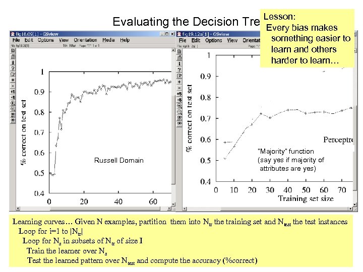Lesson: Evaluating the Decision Trees Every bias makes something easier to learn and others harder to learn… Russell Domain “Majority” function (say yes if majority of attributes are yes) Learning curves… Given N examples, partition them into Ntr the training set and Ntest the test instances Loop for i=1 to |Ntr| Loop for Ns in subsets of Ntr of size I Train the learner over Ns Test the learned pattern over Ntest and compute the accuracy (%correct)

Problems with Info. Gain. Heuristics • Feature correlation: The Costanza party problem – No obvious solution… • Overfitting: We may look too hard for patterns where there are none – E. g. Coin tosses classified by the day of the week, the shirt I was wearing, the time of the day etc. – Solution: Don’t consider splitting if the information gain given by the best feature is below a minimum threshold • Can use the c 2 test for statistical significance – Will also help when we have noisy samples… • We may prefer features with very high branching – e. g. Branch on the “universal time string” for Russell restaurant example – Branch on social security number to look for patterns on who will get A – Solution: “gain ratio” --ratio of information gain with the attribute A to the information content of answering the question “What is the value of A? ” • The denominator is smaller for attributes with smaller domains.

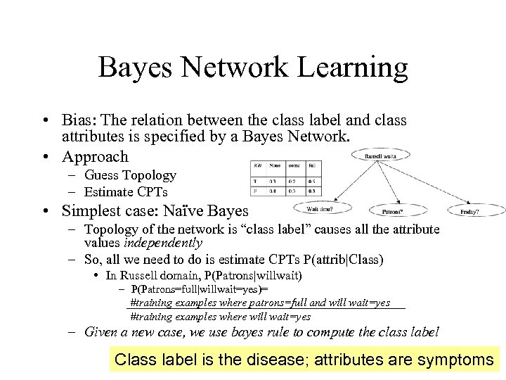Bayes Network Learning • Bias: The relation between the class label and class attributes is specified by a Bayes Network. • Approach – Guess Topology – Estimate CPTs • Simplest case: Naïve Bayes – Topology of the network is “class label” causes all the attribute values independently – So, all we need to do is estimate CPTs P(attrib|Class) • In Russell domain, P(Patrons|willwait) – P(Patrons=full|willwait=yes)= #training examples where patrons=full and will wait=yes #training examples where will wait=yes – Given a new case, we use bayes rule to compute the class label Class label is the disease; attributes are symptoms

Naïve Bayesian Classification • Problem: Classify a given example E into one of the classes among [C 1, C 2 , …, Cn] – E has k attributes A 1, A 2 , …, Ak and each Ai can take d different values • Bayes Classification: Assign E to class Ci that maximizes P(Ci | E) P(Ci| E) = P(E| Ci) P(Ci) / P(E) • P(Ci) and P(E) are a priori knowledge (or can be easily extracted from the set of data) • Estimating P(E|Ci) is harder – Requires P(A 1=v 1 A 2=v 2…. Ak=vk|Ci) • Assuming d values per attribute, we will need ndk probabilities • Naïve Bayes Assumption: Assume all attributes are independent P(E| Ci) = P P(Ai=vj | Ci ) – The assumption is BOGUS, but it seems to WORK (and needs only n*d*k probabilities

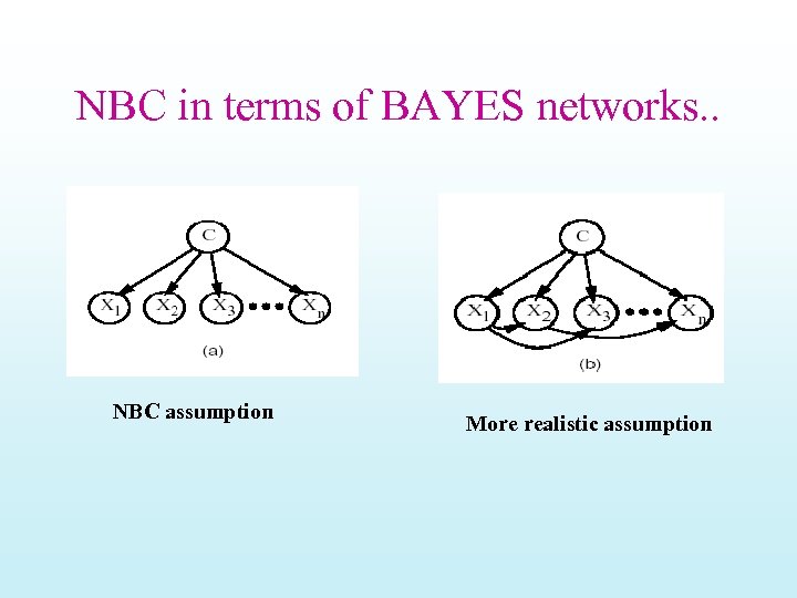NBC in terms of BAYES networks. . NBC assumption More realistic assumption

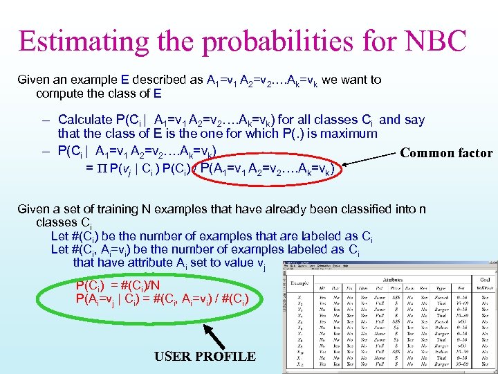Estimating the probabilities for NBC Given an example E described as A 1=v 1 A 2=v 2…. Ak=vk we want to compute the class of E – Calculate P(Ci | A 1=v 1 A 2=v 2…. Ak=vk) for all classes Ci and say that the class of E is the one for which P(. ) is maximum – P(Ci | A 1=v 1 A 2=v 2…. Ak=vk) Common factor = P P(vj | Ci ) P(Ci) / P(A 1=v 1 A 2=v 2…. Ak=vk) Given a set of training N examples that have already been classified into n classes Ci Let #(Ci) be the number of examples that are labeled as Ci Let #(Ci, Ai=vi) be the number of examples labeled as Ci that have attribute Ai set to value vj P(Ci) = #(Ci)/N P(Ai=vj | Ci) = #(Ci, Ai=vi) / #(Ci) USER PROFILE

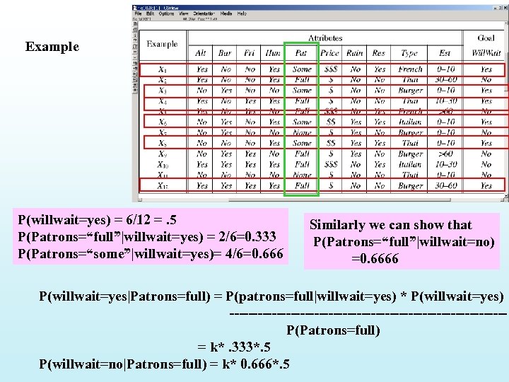
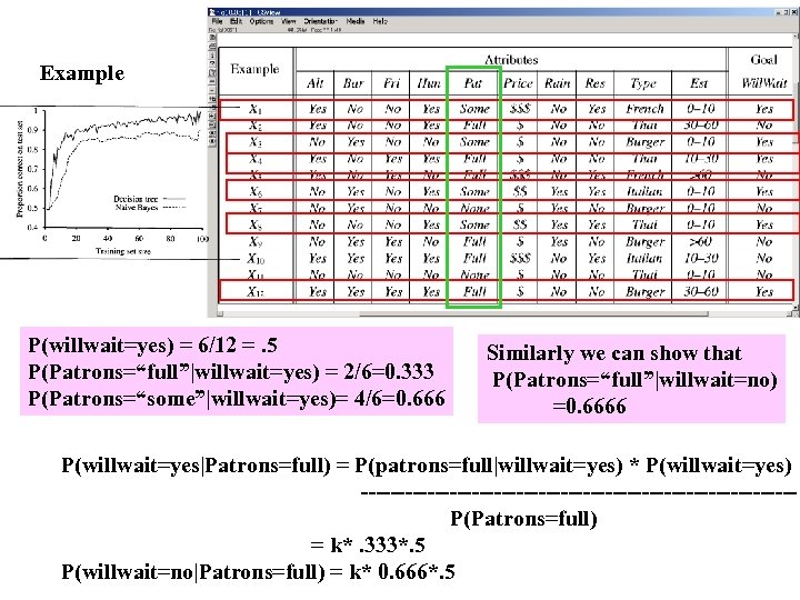Example P(willwait=yes) = 6/12 =. 5 P(Patrons=“full”|willwait=yes) = 2/6=0. 333 P(Patrons=“some”|willwait=yes)= 4/6=0. 666 Similarly we can show that P(Patrons=“full”|willwait=no) =0. 6666 P(willwait=yes|Patrons=full) = P(patrons=full|willwait=yes) * P(willwait=yes) -----------------------------P(Patrons=full) = k*. 333*. 5 P(willwait=no|Patrons=full) = k* 0. 666*. 5

Using M-estimates to improve probablity estimates • The simple frequency based estimation of P(Ai=vj|Ck) can be inaccurate, especially when the true value is close to zero, and the number of training examples is small (so the probability that your examples don’t contain rare cases is quite high) • Solution: Use M-estimate P(Ai=vj | Ci) = [#(Ci, Ai=vi) + mp ] / [#(Ci) + m] – p is the prior probability of Ai taking the value vi • If we don’t have any background information, assume uniform probability (that is 1/d if Ai can take d values) – m is a constant—called “equivalent sample size” • If we believe that our sample set is large enough, we can keep m small. Otherwise, keep it large. • Essentially we are augmenting the #(Ci) normal samples with m more virtual samples drawn according to the prior probability on how Ai takes values – Popular values p=1/|V| and m=|V| where V is the size of the vocabulary Also, to avoid overflow errors do addition of logarithms of probabilities (instead of multiplication of probabilities)

How Well (and WHY) DOES NBC WORK? • Naïve bayes classifier is darned easy to implement – Good learning speed, classification speed – Modest space storage – Supports incrementality • It seems to work very well in many scenarios – Lots of recommender systems (e. g. Amazon books recommender) use it – Peter Norvig, the director of Machine Learning at GOOGLE said, when asked about what sort of technology they use “Naïve bayes” • But WHY? – NBC’s estimate of class probability is quite bad • BUT classification accuracy is different from probability estimate accuracy – [Domingoes/Pazzani; 1996] analyze this

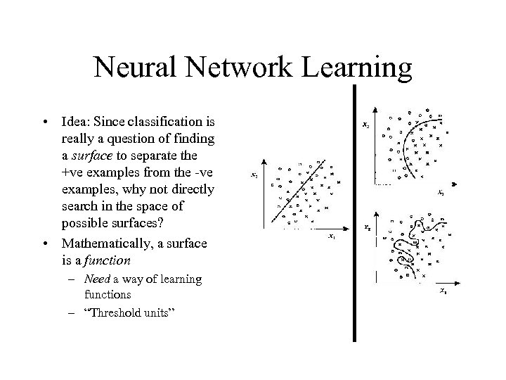Neural Network Learning • Idea: Since classification is really a question of finding a surface to separate the +ve examples from the -ve examples, why not directly search in the space of possible surfaces? • Mathematically, a surface is a function – Need a way of learning functions – “Threshold units”

“Neural Net” is a collection of threshold units with interconnections differentiable = 1 if w 1 I 1+w 2 I 2 > k = 0 otherwise Recurrent Feed Forward Single Layer Uni-directional connections Any linear decision surface can be represented by a single layer neural net Multi-Layer Any “continuous” decision surface (function) can be approximated to any degree of accuracy by some 2 -layer neural net Bi-directional connections Can act as associative memory

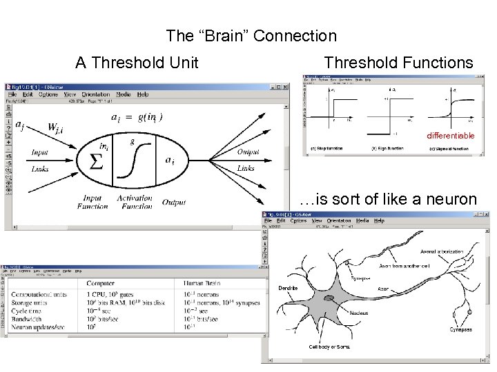The “Brain” Connection A Threshold Unit Threshold Functions differentiable …is sort of like a neuron

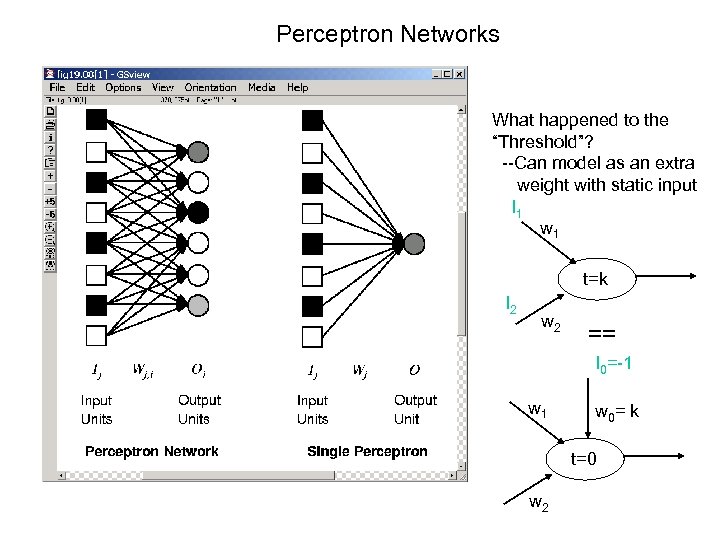Perceptron Networks What happened to the “Threshold”? --Can model as an extra weight with static input I 1 w 1 t=k I 2 w 2 == I 0=-1 w 0 = k t=0 w 2

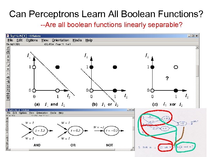Can Perceptrons Learn All Boolean Functions? --Are all boolean functions linearly separable?

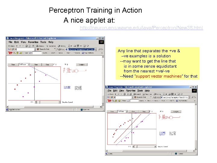Perceptron Training in Action A nice applet at: http: //neuron. eng. wayne. edu/java/Perceptron/New 38. html Any line that separates the +ve & –ve examples is a solution --may want to get the line that is in some sense equidistant from the nearest +ve/-ve --Need “support vector machines” for that

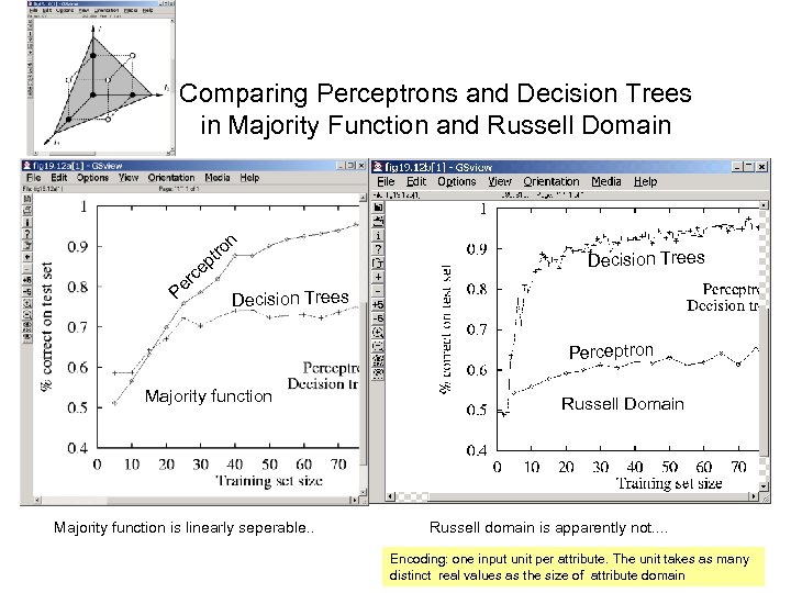Comparing Perceptrons and Decision Trees in Majority Function and Russell Domain n tro p e rc e P Decision Trees Perceptron Majority function is linearly seperable. . Russell Domain Russell domain is apparently not. . Encoding: one input unit per attribute. The unit takes as many distinct real values as the size of attribute domain

Neural Nets Continued. .

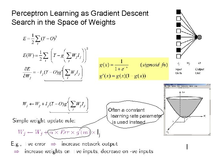Perceptron Learning as Gradient Descent Search in the Space of Weights Often a constant learning rate parameter is used instead Ij I

Perceptron Training in Action A nice applet at: http: //neuron. eng. wayne. edu/java/Perceptron/New 38. html Any line that separates the +ve & –ve examples is a solution --may want to get the line that is in some sense equidistant from the nearest +ve/-ve --Need “support vector machines” for that

Comparing Perceptrons and Decision Trees in Majority Function and Russell Domain n tro p e rc e P Decision Trees Perceptron Majority function is linearly seperable. . Russell Domain Russell domain is apparently not. . Encoding: one input unit per attribute. The unit takes as many distinct real values as the size of attribute domain

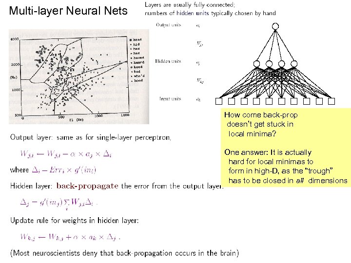Multi-layer Neural Nets How come back-prop doesn’t get stuck in local minima? One answer: It is actually hard for local minimas to form in high-D, as the “trough” has to be closed in all dimensions

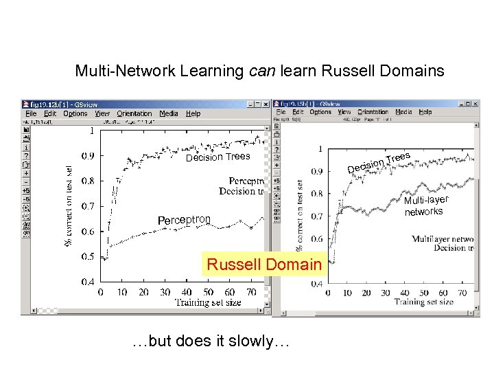Multi-Network Learning can learn Russell Domains Decision Trees Perceptron Russell Domain …but does it slowly… rees on T ecisi D Multi-layer networks

Practical Issues in Multi-layer network learning • For multi-layer networks, we need to learn both the weights and the network topology – Topology is fixed for perceptrons • If we go with too many layers and connections, we can get over-fitting as well as sloooow convergence – Optimal brain damage • Start with more than needed hidden layers as well as connections; after a network is learned, remove the nodes and connections that have very low weights; retrain

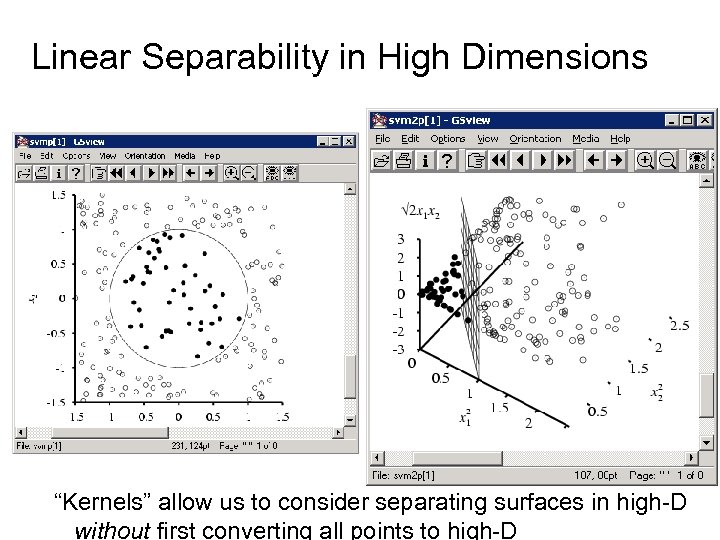Linear Separability in High Dimensions “Kernels” allow us to consider separating surfaces in high-D without first converting all points to high-D

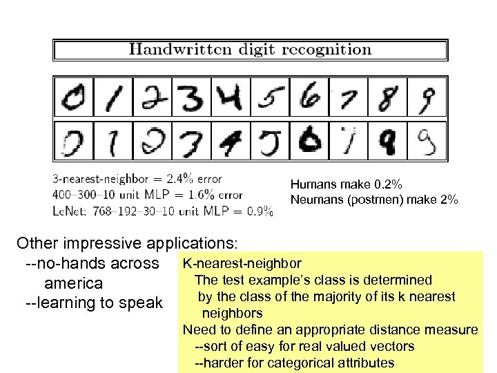Humans make 0. 2% Neumans (postmen) make 2% Other impressive applications: --no-hands across K-nearest-neighbor The test example’s class is determined america by the class of the majority of its k nearest --learning to speak neighbors Need to define an appropriate distance measure --sort of easy for real valued vectors --harder for categorical attributes

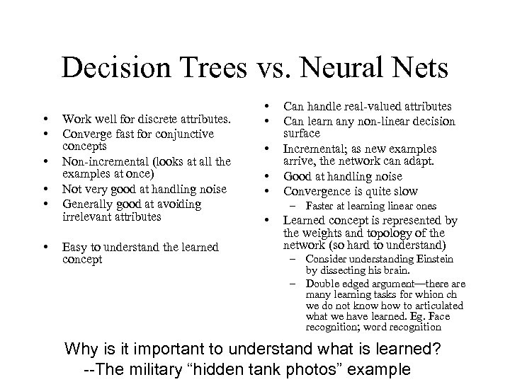Decision Trees vs. Neural Nets • • • Work well for discrete attributes. Converge fast for conjunctive concepts Non-incremental (looks at all the examples at once) Not very good at handling noise Generally good at avoiding irrelevant attributes Easy to understand the learned concept • • • Can handle real-valued attributes Can learn any non-linear decision surface Incremental; as new examples arrive, the network can adapt. Good at handling noise Convergence is quite slow – Faster at learning linear ones • Learned concept is represented by the weights and topology of the network (so hard to understand) – Consider understanding Einstein by dissecting his brain. – Double edged argument—there are many learning tasks for whion ch we do not know how to articulated what we have learned. Eg. Face recognition; word recognition Why is it important to understand what is learned? --The military “hidden tank photos” example

Example P(willwait=yes) = 6/12 =. 5 P(Patrons=“full”|willwait=yes) = 2/6=0. 333 P(Patrons=“some”|willwait=yes)= 4/6=0. 666 Similarly we can show that P(Patrons=“full”|willwait=no) =0. 6666 P(willwait=yes|Patrons=full) = P(patrons=full|willwait=yes) * P(willwait=yes) -----------------------------P(Patrons=full) = k*. 333*. 5 P(willwait=no|Patrons=full) = k* 0. 666*. 5

Feature Selection • • A problem -- too many features -- each vector x contains “several thousand” features. – Most come from “word” features -- include a word if any e-mail contains it (eg, every x contains an “opossum” feature even though this word occurs in only one message). – Slows down learning and predictoins – May cause lower performance • The Naïve Bayes Classifier makes a huge assumption -- the “independence” assumption. • A good strategy is to have few features, to minimize the chance that the assumption is violated. • Ideally, discard all features that violate the assumption. (But if we knew these features, we wouldn’t need to make the naive independence assumption!) Feature selection: “a few thousand” 500 features

Feature-Selection approach • Lots of ways to perform feature selection – FEATURE SELECTION ~ DIMENSIONALITY REDUCTION • • One simple strategy: mutual information Suppose we have two random variables A and B. Mutual information MI(A, B) is a numeric measure of what we can conclude about A if we know B, and vice-versa. MI(A, B) = Pr(A&B) log(Pr(A&B)/(Pr(A)Pr(B))) – Example: If A and B are independent, then we can’t conclude anything: MI(A, B) = 0 • Note that MI can be calculated without needing conditional probabilities.

Mutual Information, continued – Check our intuition: independence -> MI(A, B)=0 MI(A, B) = Pr(A&B) log(Pr(A&B)/(Pr(A)Pr(B))) = Pr(A&B) log(Pr(A)Pr(B)/(Pr(A)Pr(B))) = Pr(A&B) log 1 = 0 – Fully correlated, it becomes the “information content” • MI(A, A)= - Pr(A)log(Pr(A)) – {it depends on how “uncertain” the event is; notice that the expression becomes maximum (=1) when Pr(A)=. 5; this makes sense since the most uncertain event is one whose probability is. 5 (if it is. 3 then we know it is likely not to happen; if it is. 7 we know it is likely to happen).

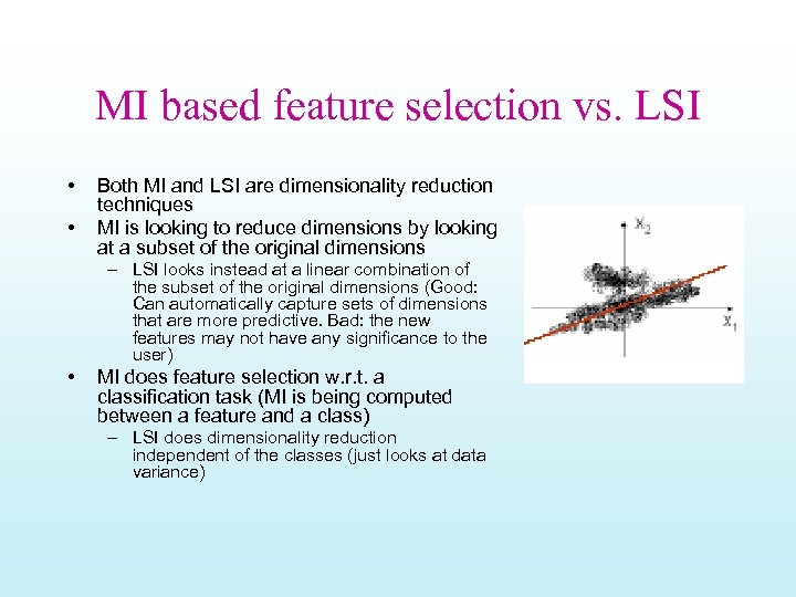MI based feature selection vs. LSI • • Both MI and LSI are dimensionality reduction techniques MI is looking to reduce dimensions by looking at a subset of the original dimensions – LSI looks instead at a linear combination of the subset of the original dimensions (Good: Can automatically capture sets of dimensions that are more predictive. Bad: the new features may not have any significance to the user) • MI does feature selection w. r. t. a classification task (MI is being computed between a feature and a class) – LSI does dimensionality reduction independent of the classes (just looks at data variance)

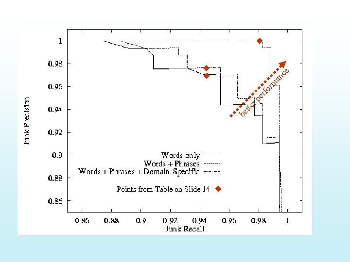
Experiments • 1789 hand-tagged e-mail messages – 1578 junk – 211 legit • Split into… – 1528 training messages (86%) – 251 testing messages (14%) – Similar to experiment described in Ad. Eater lecture, except messages are not randomly split. This is unfortunate -maybe performance is just a fluke. • Training phase: Compute Pr[X=x|C=junk], Pr[X=x], and P[C=junk] from training messages • Testing phase: Compute Pr[C=junk|X=x] for each training message x. Predict “junk” if Pr[C=junk|X=x]>0. 999. Record mistake/correct answer in confusion matrix.

be tte rp er fo rm an ce Precision/Recall Curves Points from Table on Slide 14

Note that all features—whether words, phrases or domain names etc are Treated the same way—we estimate P(feature|class) probabilities and use them Sahami et. Al. spam filtering • The above framework is completely general. We just need to encode each e-mail as a fixed-width vector X = X 1, X 2, X 3, . . . , generated XN of features. automatically • So. . . What features are used in Sahami’s system – words – suggestive phrases (“free money”, “must be over 21”, . . . ) hand – sender’s domain (. com, . edu, . gov, . . . ) crafted! – peculiar punctuation (“!!!Get Rich Quick!!!”) – did email contain an attachment? – was message sent during evening or daytime? – ? • (We’ll see a similar list for Ad. Eater and other learning systems)

How Well (and WHY) DOES NBC WORK? • Naïve bayes classifier is darned easy to implement • Good learning speed, classification speed • Modest space storage • Supports incrementality – Recommendations re-done as more attribute values of the new item become known. • It seems to work very well in many scenarios – Peter Norvig, the director of Machine Learning at GOOGLE said, when asked about what sort of technology they use “Naïve bayes” • But WHY? – [Domingos/Pazzani; 1996] showed that NBC has much wider ranges of applicability than previously thought (despite using the independence assumption) – classification accuracy is different from probability estimate accuracy • Notice that normal classification application don’t quite care about the actual probability; only which probability is the highest – Exception is Cost-based learning—suppose false positives and false negatives have different costs… » E. g. Sahami et al consider a message to be spam only if Spam class probability is >. 9 (so they are using incorrect NBC estimates here)

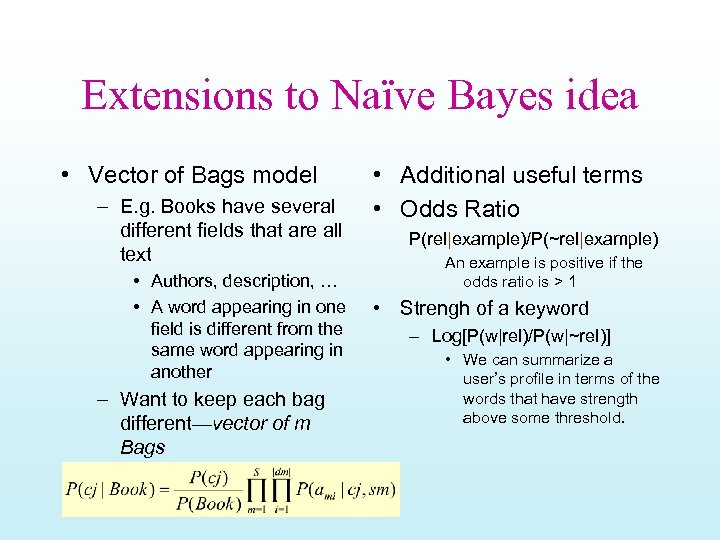Extensions to Naïve Bayes idea • Vector of Bags model – E. g. Books have several different fields that are all text • Authors, description, … • A word appearing in one field is different from the same word appearing in another – Want to keep each bag different—vector of m Bags • Additional useful terms • Odds Ratio P(rel|example)/P(~rel|example) An example is positive if the odds ratio is > 1 • Strengh of a keyword – Log[P(w|rel)/P(w|~rel)] • We can summarize a user’s profile in terms of the words that have strength above some threshold.

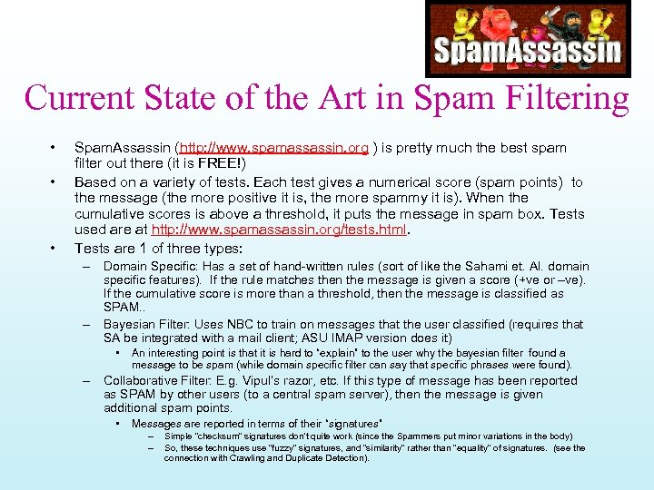Current State of the Art in Spam Filtering • • • Spam. Assassin (http: //www. spamassassin. org ) is pretty much the best spam filter out there (it is FREE!) Based on a variety of tests. Each test gives a numerical score (spam points) to the message (the more positive it is, the more spammy it is). When the cumulative scores is above a threshold, it puts the message in spam box. Tests used are at http: //www. spamassassin. org/tests. html. Tests are 1 of three types: – Domain Specific: Has a set of hand-written rules (sort of like the Sahami et. Al. domain specific features). If the rule matches then the message is given a score (+ve or –ve). If the cumulative score is more than a threshold, then the message is classified as SPAM. . – Bayesian Filter: Uses NBC to train on messages that the user classified (requires that SA be integrated with a mail client; ASU IMAP version does it) • An interesting point is that it is hard to “explain” to the user why the bayesian filter found a message to be spam (while domain specific filter can say that specific phrases were found). – Collaborative Filter: E. g. Vipul’s razor, etc. If this type of message has been reported as SPAM by other users (to a central spam server), then the message is given additional spam points. • Messages are reported in terms of their “signatures” – – Simple “checksum” signatures don’t quite work (since the Spammers put minor variations in the body) So, these techniques use “fuzzy” signatures, and “similarity” rather than “equality” of signatures. (see the connection with Crawling and Duplicate Detection).

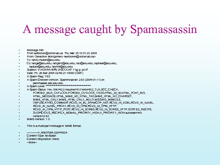A message caught by Spamassassin • • • • • • Message 346: From aetbones@ccinet. ab. ca Thu Mar 25 16: 51: 23 2004 From: Geraldine Montgomery To: randy. mullen@asu. edu Cc: ranga@asu. edu, rangers@asu. edu, rao@asu. edu, raphael@asu. edu, rapture@asu. edu, rashmi@asu. edu Subject: V 1 AGKRA 80% DISCOUNT !! sg g pz kf Date: Fri, 26 Mar 2004 02: 49: 21 +0000 (GMT) X-Spam-Flag: YES X-Spam-Checker-Version: Spam. Assassin 2. 63 (2004 -01 -11) on parichaalak. eas. asu. edu X-Spam-Level: ********************* X-Spam-Status: Yes, hits=42. 2 required=5. 0 tests=BIZ_TLD, DCC_CHECK, FORGED_MUA_OUTLOOK, FORGED_OUTLOOK_TAGS, HTML_30_40, HTML_FONT_BIG, HTML_MESSAGE, HTML_MIME_NO_HTML_TAG, MIME_HTML_NO_CHARSET, MIME_HTML_ONLY_MULTI, MISSING_MIMEOLE, OBFUSCATING_COMMENT, RCVD_IN_BL_SPAMCOP_NET, RCVD_IN_DSBL, RCVD_IN_NJABL_PROXY, RCVD_IN_OPM_HTTP, RCVD_IN_OPM_HTTP_POST, RCVD_IN_SORBS_HTTP, SORTED_RECIPS, SUSPICIOUS_RECIPS, X_MSMAIL_PRIORITY_HIGH, X_PRIORITY_HIGH autolearn=no version=2. 63 MIME-Version: 1. 0 • This is a multi-part message in MIME format. • • ------=_40637084. 02 AF 45 D 4 Content-Type: text/plain Content-Disposition: inline --More--

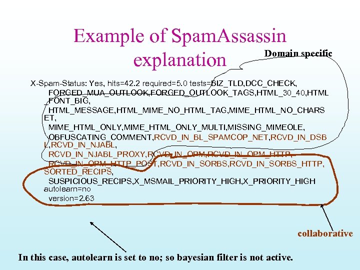Example of Spam. Assassin Domain specific explanation X-Spam-Status: Yes, hits=42. 2 required=5. 0 tests=BIZ_TLD, DCC_CHECK, FORGED_MUA_OUTLOOK, FORGED_OUTLOOK_TAGS, HTML_30_40, HTML _FONT_BIG, HTML_MESSAGE, HTML_MIME_NO_HTML_TAG, MIME_HTML_NO_CHARS ET, MIME_HTML_ONLY_MULTI, MISSING_MIMEOLE, OBFUSCATING_COMMENT, RCVD_IN_BL_SPAMCOP_NET, RCVD_IN_DSB L, RCVD_IN_NJABL_PROXY, RCVD_IN_OPM_HTTP, RCVD_IN_OPM_HTTP_POST, RCVD_IN_SORBS_HTTP, SORTED_RECIPS, SUSPICIOUS_RECIPS, X_MSMAIL_PRIORITY_HIGH, X_PRIORITY_HIGH autolearn=no version=2. 63 collaborative In this case, autolearn is set to no; so bayesian filter is not active.

General comments on Spam • • Spam is a technical problem (we created it) It has the “arms-race” character to it – We can’t quite legislate against SPAM • Most spam comes from outside national boundaries… • Need “technical” solutions – To detect Spam (we mostly have a handle on it) – To STOP spam generation (detecting spam after its gets sent still is taxing mail servers—by some estimates more than 66% of the mail relayed by AOL/Yahoo mailservers is SPAM • Brother Gates suggest “monetary” cost – Make every mailer pay for the mail they send » Not necessarily in “stamps” but perhaps by agreeing to give some CPU cycles to work on some problem (e. g. finding primes; computing PI etc) » The cost will be minuscule for normal users, but will multiply for spam mailers who send millions of mails. • Other innovative ideas needed—we now have a conferences on Spam mail – http: //www. ceas. cc/

Combining Content and Collaboration • Content-based and collaborative methods have complementary strengths and weaknesses. • Combine methods to obtain the best of both. • Various hybrid approaches: – Apply both methods and combine recommendations. – Use collaborative data as content. – Use content-based predictor as another collaborator. – Use content-based predictor to complete collaborative data.

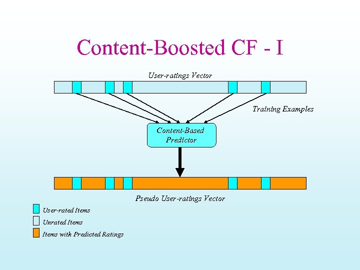Content-Boosted CF - I User-ratings Vector Training Examples Content-Based Predictor Pseudo User-ratings Vector User-rated Items Unrated Items with Predicted Ratings

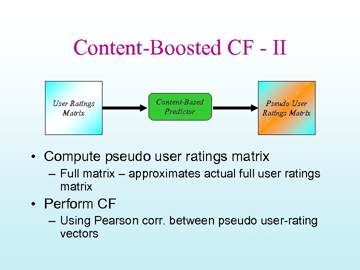Content-Boosted CF - II User Ratings Matrix Content-Based Predictor Pseudo User Ratings Matrix • Compute pseudo user ratings matrix – Full matrix – approximates actual full user ratings matrix • Perform CF – Using Pearson corr. between pseudo user-rating vectors