1 Transformation of a Drawing

1 Transformation of a Drawing Some problems can be solved easier if object has a particular location relating to the plane of projection. For instance, if a straight line segment is parallel to the plane of projection, it projects to a true size. Otherwise, to find its true length we need to use method of a right-angular triangle. To achieve this we can apply methods called Transformation of a Drawing. Three ways how to transform a drawing 1. Replacing of planes of projection (projecting to auxiliary planes) ; 2. Revolution of a model about an axes perpendicular to a plane of projection ; 3. Planar parallel motion (revolution of a model about an axes without indicating an axes in the drawing). Basic problems which can be solved by Transformation of a Drawing : Oblique line segment transforms to a line segment parallel to the plane of projection ; Oblique line segment transforms to a line segment perpendicular to the plane of projection ; Oblique plane segment transforms to a plane segment parallel to the plane of projection.

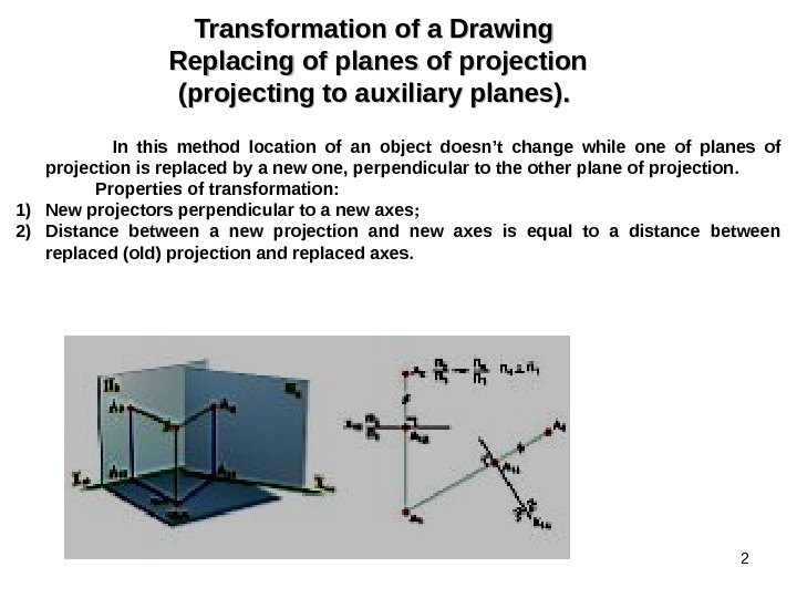
2 Transformation of a Drawing Replacing of planes of projection (projecting to auxiliary planes). . In this method location of an object doesn’t change while one of planes of projection is replaced by a new one, perpendicular to the other plane of projection. Properties of transformation : 1) New projectors perpendicular to a new axes ; 2) Distance between a new projection and new axes is equal to a distance between replaced (old) projection and replaced axes.

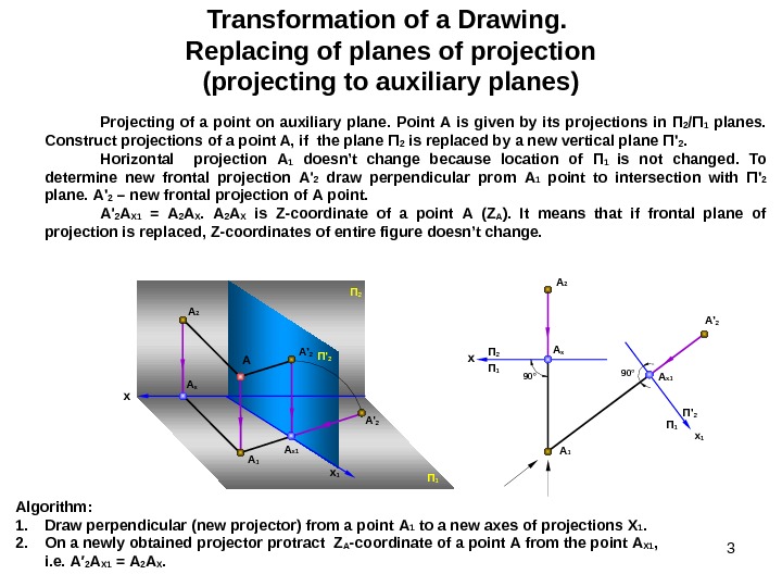
3 Transformation of a Drawing. Replacing of planes of projection (projecting to auxiliary planes) Projecting of a point on auxiliary plane. Point А is given by its projections in П 2 /П 1 planes. Construct projections of a point A, if the plane П 2 is replaced by a new vertical plane П ‘ 2. Horizontal projection А 1 doesn’t change because location of П 1 is not changed. To determine new frontal projection А ‘ 2 draw perpendicular prom А 1 point to intersection with П ‘ 2 plane. А ‘ 2 – new frontal projection of А point. А ‘ 2 А Х 1 = А 2 А Х is Z-coordinate of a point А ( Z А ). It means that if frontal plane of projection is replaced, Z-coordinates of entire figure doesn’t change. Algorithm : 1. Draw perpendicular (new projector) from a point А 1 to a new axes of projections X 1. 2. On a newly obtained projector protract Z A -coordinate of a point А from the point А Х 1 , i. е. А′ 2 А Х 1 = А 2 А Х. A x x A 2 П 1 A x A 1 90 °A 2 A x A 1 A ‘ 2 П 1 П 2 x 1 П ‘ 2 A ‘ 2 x 1 П ‘ 2 A x 1 П 1 A x 1 A ‘

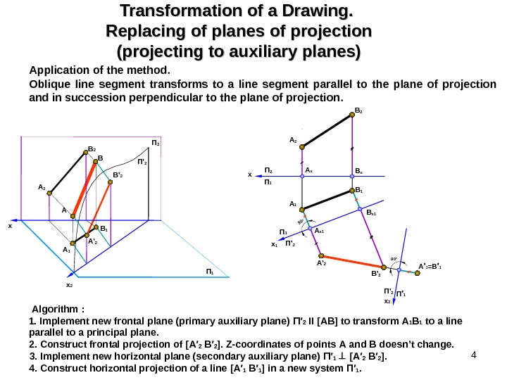
4 Transformation of a Drawing. Replacing of planes of projection (projecting to auxiliary planes) Application of the method. Oblique line segment transforms to a line segment parallel to the plane of projection and in succession perpendicular to the plane of projection. Algorithm : 1. Implement new frontal plane (primary auxiliary plane) П ′ 2 ІІ [АВ] to transform А 1 В 1 to a line parallel to a principal plane. 2. Construct frontal projection of [А′ 2 В′ 2 ]. Z-coordinates of points А and В doesn’t change. 3. Implement new horizontal plane (secondary auxiliary plane) П′ 1 [А′ 2 В′ 2 ]. 4. Construct horizontal projection of a line [А′ 1 В′ 1 ] in a new system П′ 1. x x 2 x П 2 П 1 x 1 П ‘ 2 A ‘ 1 =B ‘ 1 x 2 П ‘ 1 П ‘ 290 ° П 1 П 2 П ‘ 2 A 2 B 2 A B B’ 2 B 1 A’ 290° A x B x A x 1 B x 1 A 2 B 2 A’ 2 B’

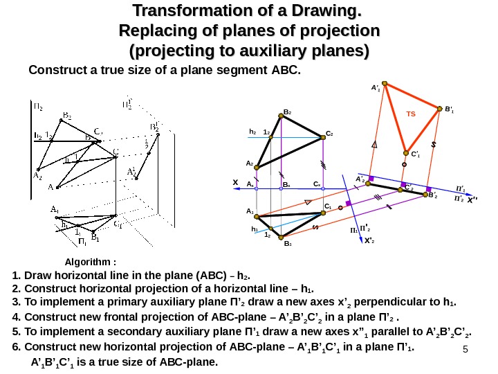
5 Transformation of a Drawing. Replacing of planes of projection (projecting to auxiliary planes) Construct a true size of a plane segment АВС. Algorithm : 1. Draw horizontal line in the plane (АВС) – h 2. 2. Construct horizontal projection of a horizontal line – h 1. 3. To implement a primary auxiliary plane П’ 2 draw a new axes x’ 2 perpendicular to h 1. 4. Construct new frontal projection of АВС -plane – A’ 2 B’ 2 C’ 2 in a plane П’ 2 . 5. To implement a secondary auxiliary plane П’ 1 draw a new axes x’’ 1 parallel to A’ 2 B’ 2 C’ 2. 6. Construct new horizontal projection of АВС -plane – A’ 1 B’ 1 C’ 1 in a plane П’ 1. A’ 1 B’ 1 C’ 1 is a true size of АВС -plane. x A 2 B 2 C x B x. A x B 1 A 1 C 11 2 h 2 x»П’2 П’1 h 1 A’1 B’1 C’1 A’2 C’2 B’2 1 2 П ‘ 2 x ‘ 2 П 1 TS

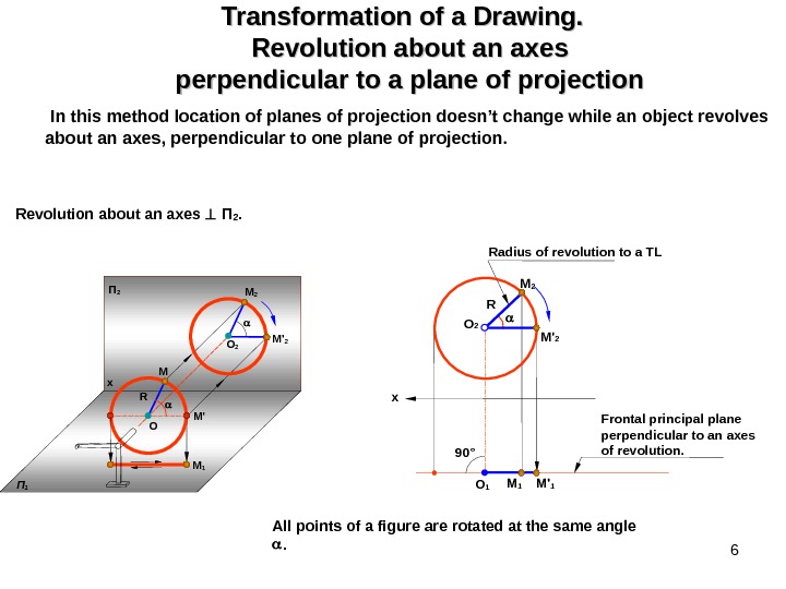
6 Transformation of a Drawing. Revolution about an axes perpendicular to a plane of projection In this method location of planes of projection doesn’t change while an object revolves about an axes, perpendicular to one plane of projection. Revolution about an axes П 2. All points of a figure are rotated at the same angle . M’ O M R O 2 M ‘ 2 x П 2 П 1 M 1 R x O 2 M 1 M ‘ 1 O 1 M 2 M ‘ 2 90° Radius of revolution to a TL Frontal principal plane perpendicular to an axes of revolution.

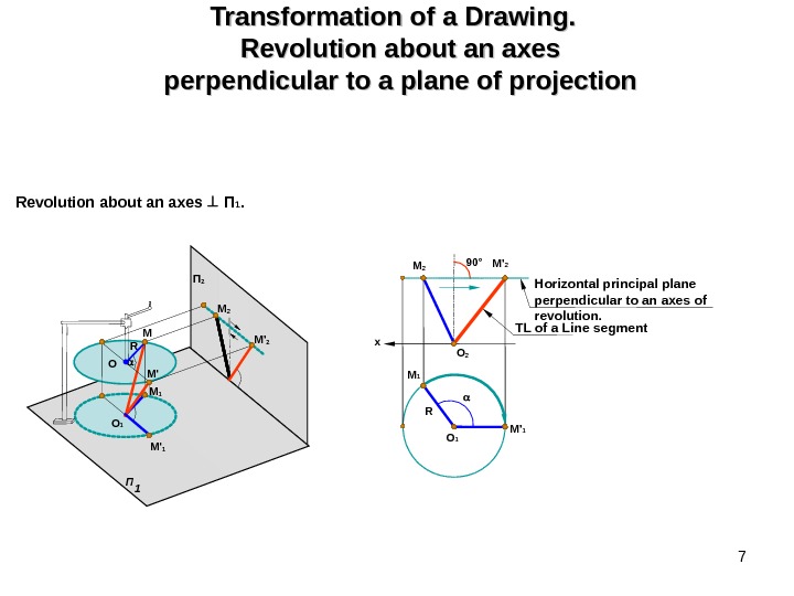
7 Transformation of a Drawing. Revolution about an axes perpendicular to a plane of projection Revolution about an axes П 1. O 1 RM 1 O 2 M 2 90° M ‘ 2 M ‘ 1 TL of a Line segment Horizontal principal plane perpendicular to an axes of revolution. x. M П 1 O 1 O R П 2 M ‘ 1 M

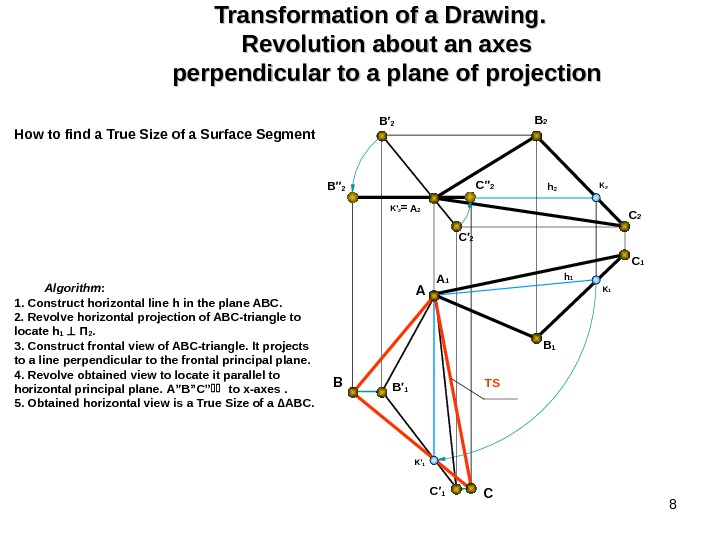
8 Transformation of a Drawing. Revolution about an axes perpendicular to a plane of projection B 2 A 2 C 2 B 1 h 2 A 1 C 1 C′ 2 h 1 B′ 1 C′ 1 B′′ 2 C′′ 2 B A CK′ 1 K 2 K 1 B′ 2 K ‘ 2 = TSHow to find a True Size of a Surface Segment Algorithm : 1. Construct horizontal line h in the plane ABC. 2. Revolve horizontal projection of ABC-triangle to locate h 1 П 2. 3. Construct frontal view of ABC-triangle. It projects to a line perpendicular to the frontal principal plane. 4. Revolve obtained view to locate it parallel to horizontal principal plane. A”B”C” to x-axes . 5. Obtained horizontal view is a True Size of a ∆ ABC.

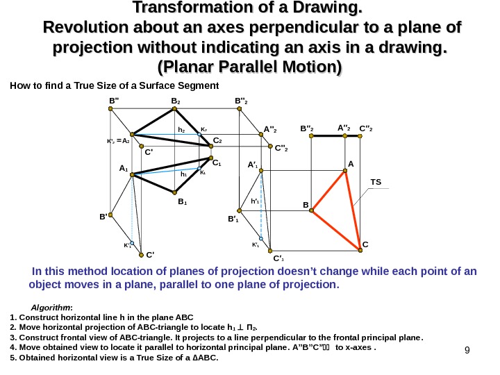
9 Transformation of a Drawing. Revolution about an axes perpendicular to a plane of projection without indicating an axis in a drawing. . (Planar Parallel Motion) How to find a True Size of a Surface Segment Algorithm : 1. Construct horizontal line h in the plane ABC 2. Move horizontal projection of ABC-triangle to locate h 1 П 2. 3. Construct frontal view of ABC-triangle. It projects to a line perpendicular to the frontal principal plane. 4. Move obtained view to locate it parallel to horizontal principal plane. A”B”C” to x-axes . 5. Obtained horizontal view is a True Size of a ∆ ABC. B 2 A 2 C 2 B 1 TSh 2 A 1 C 1 C’ h 1 h′ 1 K′ 1 B » 2 A » 2 C » 2 B A B’ C’ B′ 1 C′ 1 B′′ 2 A′′ 2 CK′ 1 K 2 K 1 A′ 1 B» K ‘ 2 = In this method location of planes of projection doesn’t change while each point of an object moves in a plane, parallel to one plane of projection.

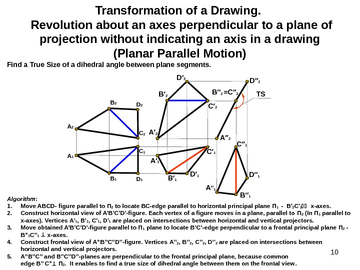
10 Transformation of a Drawing. Revolution about an axes perpendicular to a plane of projection without indicating an axis in a drawing (Planar Parallel Motion) Find a True Size of a dihedral angle between plane segments. Algorithm : 1. Move ABCD- figure parallel to П 2 to locate ВС -edge parallel to horizontal principal plane П 1 — В′ 2 C ′ 2 x-axes. 2. Construct horizontal view of A’B’C’D’-figure. Each vertex of a figure moves in a plane, parallel to П 2 (In П 1 parallel to х -axes). Vertices А’ 1 , В’ 1 , C′ 1 , D ′ 1 are placed on intersections between horizontal and vertical projectors. 3. Move obtained A’B’C’D’-figure parallel to П 1 plane to locate В ’ С ’-edge perpendicular to a frontal principal plane П 2 — В ” 1 C” 1 x-axes. 4. Construct frontal view of A”B’’C’’D’’-figure. Vertices А’ ’ 2 , В ’ ’ 2 , C ’ ′ 2 , D’ ′ 2 are placed on intersections between horizontal and vertical projectors. 5. A”B’’C’’ and B’’C’’D’’-planes are perpendicular to the frontal principal plane, because common edge В ” C” П 2. It enables to find a true size of dihedral angle between them on the frontal view. TS B 2 D 2 A 1 B 1 D 1 С 2 С 1 B′ 2 D′ 2 C′ 2 A′ 1 B′ 1 D′ 1 C′ 1 B′′ 2 =C′′ 2 D′′ 2 C′′ 1 B′′ 1 A′′ 2 A ′′ 1 D′′

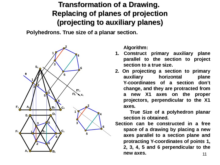
11 Transformation of a Drawing. Replacing of planes of projection (projecting to auxiliary planes) Polyhedrons. True size of a planar section. Algorithm : 1. Construct primary auxiliary plane parallel to the section to project section to a true size. 2. On projecting a section to primary auxiliary horizontal plane Y-coordinates of a section don’t change, and they are protracted from a new X 1 axes on the proper projectors, perpendicular to the X 1 axes. True Size of a polyhedron planar section is obtained. Section can be constructed in a free space of a drawing by placing a new axes parallel to a section plane and protracting Y-coordinates of points 1, 2, 3, 4, 5 and 6 perpendicular to the new axes. S 1 A 1 E 1 F 2 C 1 C 2 D 1 S 2 A 2 B 1 F 1 x 1 П ‘ 1 П

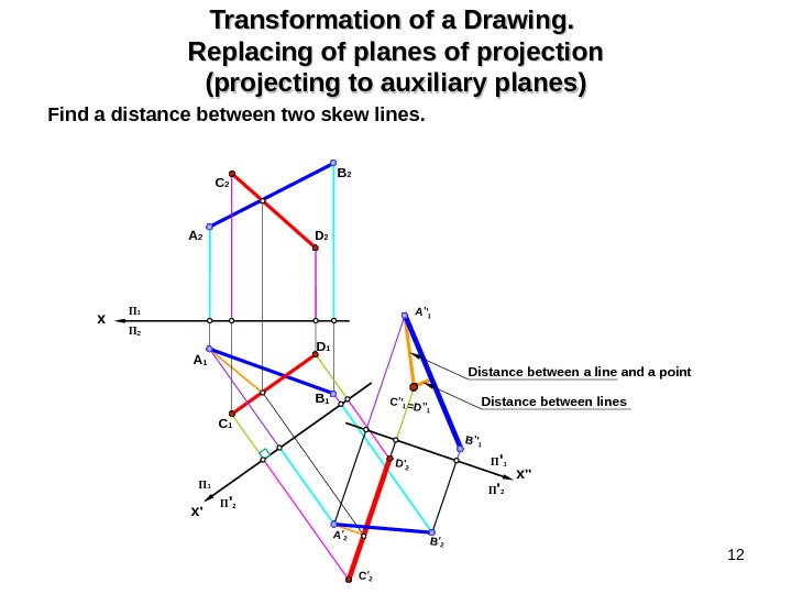
12 Transformation of a Drawing. Replacing of planes of projection (projecting to auxiliary planes) Find a distance between two skew lines. B 2 D 2 A 2 A 1 B 1 D 1 С 2 С 1 П ‘ 2 x ‘П 1 C’2 A’2 D’2 B’2 x П 1 П 2 x »П ‘ 1 П ‘ 2 Distance between lines C»1=D»1 A»1 B»1 Distance between a line and a point

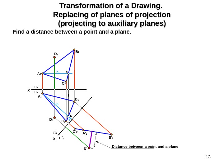
13 Transformation of a Drawing. Replacing of planes of projection (projecting to auxiliary planes) Find a distance between a point and a plane. B 2 D 2 A 1 B 1 D 1 С 2 С 1 D’ 2 C’ 2 A’ 2 B’ 2 x П 1 П 2 П ‘ 2 x ‘П 1 h 2 1 2 h 1 1 1 Distance between a point and a plane

14 Intersection between planes

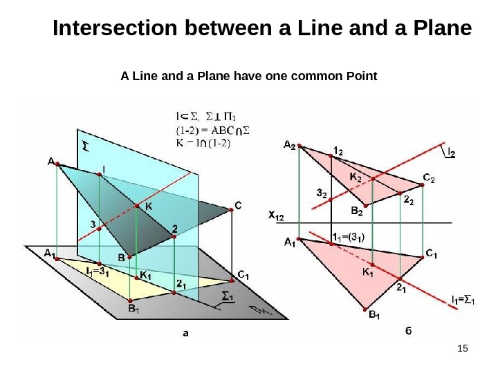
15 Intersection between a Line and a Plane A Line and a Plane have one common Point

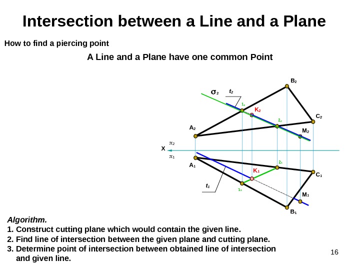
16 K 2 C 1 B 1 A 1 Intersection between a Line and a Plane A Line and a Plane have one common Point Algorithm. 1. Construct cutting plane which would contain the given line. 2. Find line of intersection between the given plane and cutting plane. 3. Determine point of intersection between obtained line of intersection and given line. How to find a piercing point X M 2 A 2 C 2 B 2 M 1 t 1 t 2 K

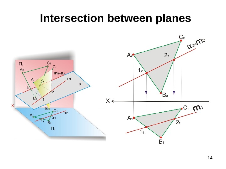
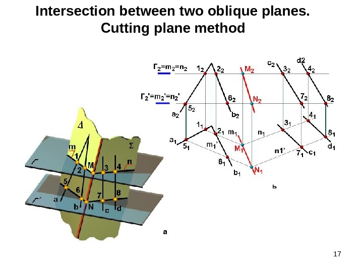
17 Intersection between two oblique planes. Cutting plane method

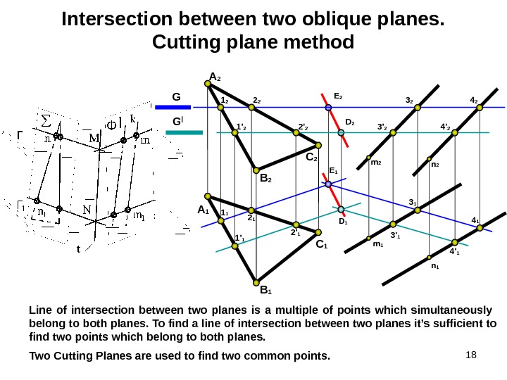
18 Intersection between two oblique planes. Cutting plane method Line of intersection between two planes is a multiple of points which simultaneously belong to both planes. To find a line of intersection between two planes it’s sufficient to find two points which belong to both planes. G G | A 2 B 2 С 2 m 1 n 1 n 2 B 1 С 1 A 1 D 2 E 2 E 1 1 1 2 1 3 1 4 1 D 1 1′ 1 2′ 1 3′ 1 4′ 11′ 2 2′ 2 3′ 2 4′ 21 2 2 2 3 2 4 2 Two Cutting Planes are used to find two common points.

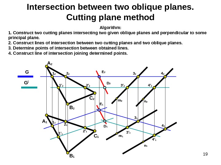
19 Intersection between two oblique planes. Cutting plane method G G | A 2 B 2 С 2 m 1 n 1 n 2 Algorithm : 1. Construct two cutting planes intersecting two given oblique planes and perpendicular to some principal plane. 2. Construct lines of intersection between two cutting planes and two oblique planes. 3. Determine points of intersection between obtained lines. 4. Construct line of intersection joining determined points. B 1 С 1 A 1 D 1 1′ 1 2′ 1 3′ 1 4′ 11′ 2 2′ 2 3′ 2 4′

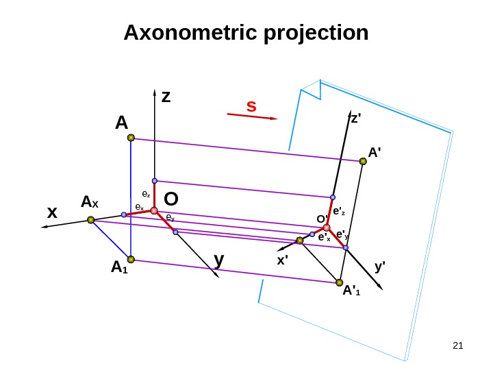
20 Axonometric projection The word ‘axonometry’ (Greek) consists of two words: ‘axon’—axis and ‘metreo’—I measure, and means ‘measuring with the aid of axes’, or ‘measuring along axes’. The method of axonometric projection consists in the fact that an object is referred to some coordinate system and then is projected by parallel lines or rays onto a plane together with the system of coordinates. Axonometric projections differ from orthographic (orthogonal) projections in that in axonometry an object is projected only onto one plane of projection called the axonometric (or pictorial ) plane and is placed in front of the picture plane so as to expose three sides to the viewer. In mechanical engineering axonometric projections are used as an auxiliary to orthographic projections of a mechanical part when it is the necessary to give a clearer picture of its shapes which are difficult to imagine from the orthographic projections. Without the axonometric picture it is sometimes very difficult to visualize the shape of the object from the three orthographic projections alone. The basic statement of axonometry» was formulated by K. Polke (in 1851) in the form of the following theorem: any three line segments emanating from a single point in the plane may be taken as a parallel projection of three equal and mutually perpendicular line segments in space. In the sixties of the 19 -th century G. Schwartz generalized Polke’s theorem. He proved that any complete quadrilateral in the plane may always be regarded as a parallel projection of a tetrahedron similar to any given one. Therefore, any three non-coincident straight lines passing through a point in the plane may be taken for the axonometric axes with various scales.

21 y’x’ z’Axonometric projection A 1 x A X A O sz y A ‘ 1 A ‘ e ‘ x e ‘ z e ‘ y. O ‘e x e z e y

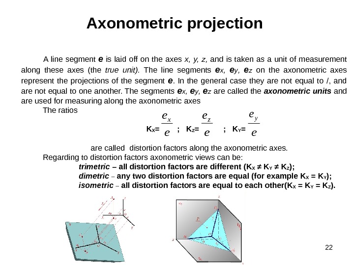
22 Axonometric projection A line segment e is laid off on the axes x, y, z, and is taken as a unit of measurement along these axes (the true unit). The line segments e x , e y , e z on the axonometric axes represent the projections of the segment e. In the general case they are not equal to /, and are not equal to one another. The segments e x , e y , e z are called the axonometric units and are used for measuring along the axonometric axes The ratios K X = ; K Z = ; K Y = are called distortion factors along the axonometric axes. Regarding to distortion factors axonometric views can be: trimetric – all distortion factors are different ( K X ≠ K Y ≠ K Z ); dimetric – any two distortion factors are equal ( for example K X = K Y ); isometric – all distortion factors are equal to each other ( K X = K Y = K Z ). e ex e ez e ey

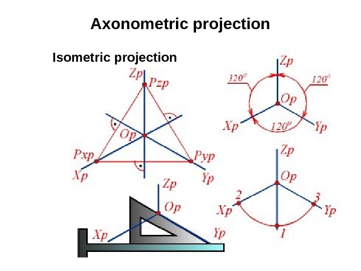
23 Axonometric projection Isometric projection

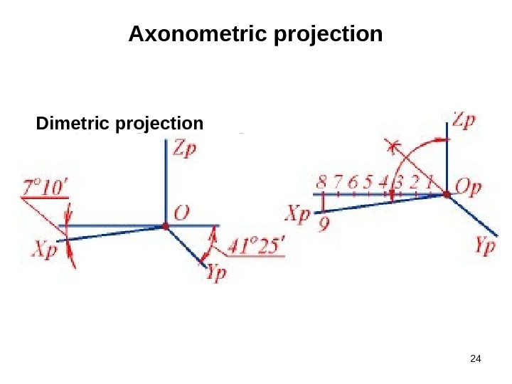
24 Axonometric projection Dimetric projection

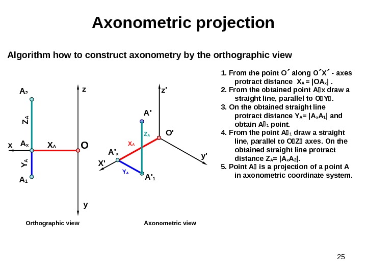
251. From the point О along О Х — axes protract distance X A = | ОA x | . 2. From the obtained point A x draw a straight line , parallel to О Y . 3. On the obtained straight line protract distance Y A = | A x A 1 | and obtain А 1 point. 4. From the point А 1 draw a straight line , parallel to O Z axes. On the obtained straight line protract distance Z A = | A x A 2 |. 5. Point А is a projection of a point А in axonometric coordinate system. Algorithm how to construct axonometry by the orthographic view Axonometric projection Axonometric view. Orthographic viewx y. OA 2 z O ‘ A 1 X AZA Y AA x X’ z’ y’ Y A A ‘ 1 X A A ‘ x Z AA ‘

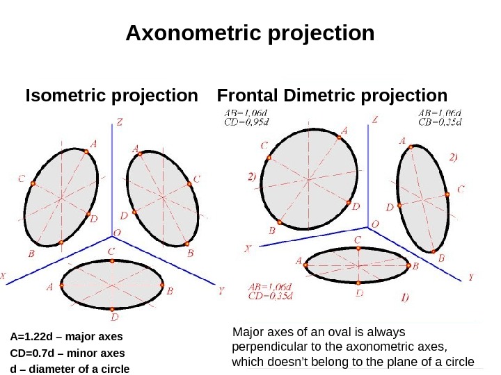
26 Axonometric projection Isometric projection Frontal Dimetric projection A=1. 22 d – major axes CD=0. 7 d – minor axes d – diameter of a circle Major axes of an oval is always perpendicular to the axonometric axes, which doesn’t belong to the plane of a circle

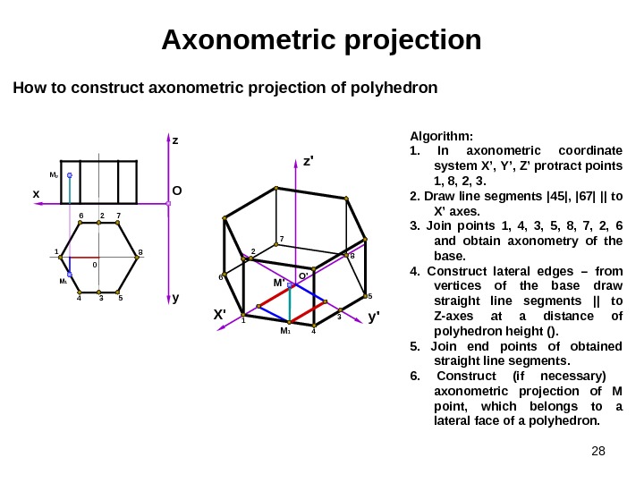
28 Axonometric projection Algorithm : 1. In axonometric coordinate system X ’, Y ’, Z ’ protract points 1, 8, 2, 3. 2. Draw line segments | 45 | , | 67 | || to X ’ axes. 3. Join points 1, 4, 3, 5, 8, 7, 2, 6 and obtain axonometry of the base. 4. Construct lateral edges – from vertices of the base draw straight line segments || to Z-axes at a distance of polyhedron height (). 5. Join end points of obtained straight line segments. 6. Construct (if necessary) axonometric projection of М point , which belongs to a lateral face of a polyhedron. How to construct axonometric projection of polyhedron O ‘ X’ z’ y’ 1 8 6 7 4 5 yz O x 1 4 3 5 8726 M 1 M 2 0 M’ 32 M

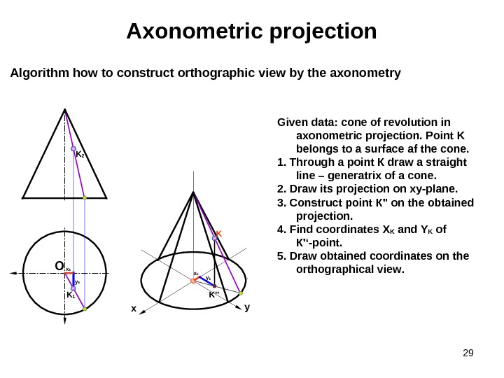
29 Axonometric projection Algorithm how to construct orthographic view by the axonometry Given data : cone of revolution in axonometric projection. Point K belongs to a surface af the cone. 1. Through a point К draw a straight line – generatrix of a cone. 2. Draw its projection on xy-plane. 3. Construct point К » on the obtained projection. 4. Find coordinates Х K and Y K of К ‘‘-point. 5. Draw obtained coordinates on the orthographical view. O x y. KK 2 x k y kx k K 1 K»

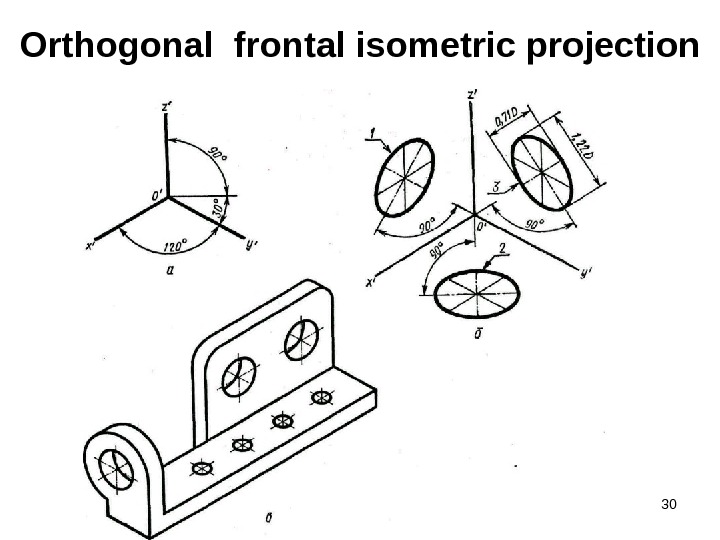
30 Orthogonal frontal isometric projection

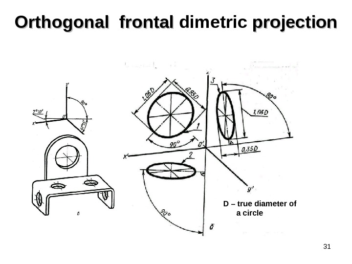
31 Orthogonal frontal dimetric projection D – true diameter of a circle

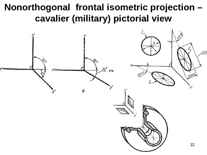
32 Nonorthogonal frontal isometric projection – cavalier (military) pictorial view

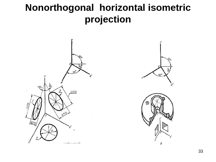
33 Nonorthogonal horizontal isometric projection

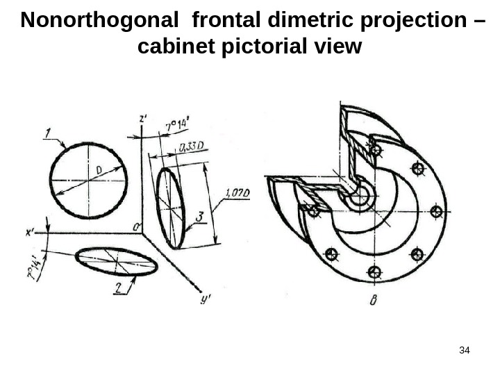
34 Nonorthogonal frontal dimetric projection – cabinet pictorial view