6c9413d5283a48b504a47e4db39cb14d.ppt
- Количество слайдов: 36

1 Technical Note 8 Process Capability and Statistical Quality Control Mc. Graw-Hill/Irwin ©The Mc. Graw-Hill Companies, Inc. , 2006
2 OBJECTIVES Process Variation Process Capability Process Control Procedures – – Variable data Attribute data Acceptance Sampling – Mc. Graw-Hill/Irwin Operating Characteristic Curve © 2006 The Mc. Graw-Hill Companies, Inc. , All Rights Reserved.
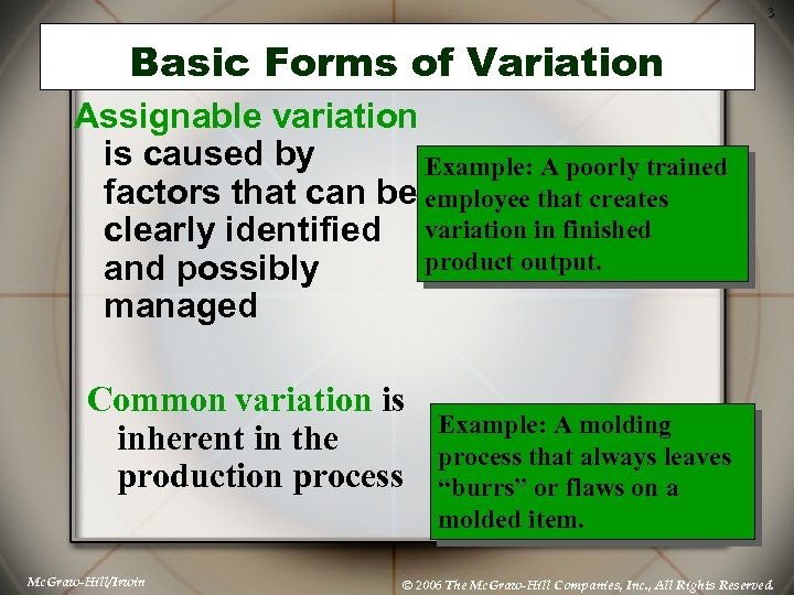
3 Basic Forms of Variation Assignable variation is caused by Example: A poorly trained factors that can be employee that creates clearly identified variation in finished product output. and possibly managed Common variation is inherent in the production process Mc. Graw-Hill/Irwin Example: A molding process that always leaves “burrs” or flaws on a molded item. © 2006 The Mc. Graw-Hill Companies, Inc. , All Rights Reserved.
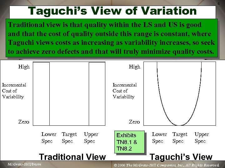
Taguchi’s View of Variation 4 Traditional view is that quality within the LS and US is good and that the cost of quality outside this range is constant, where Taguchi views costs as increasing as variability increases, so seek to achieve zero defects and that will truly minimize quality costs. High Incremental Cost of Variability Zero Lower Spec Target Spec Upper Spec Traditional View Mc. Graw-Hill/Irwin Exhibits TN 8. 1 & TN 8. 2 Lower Spec Target Spec Upper Spec Taguchi’s View © 2006 The Mc. Graw-Hill Companies, Inc. , All Rights Reserved.
Process Capability Process limits Specification limits 5 How do the limits relate to one another? Mc. Graw-Hill/Irwin © 2006 The Mc. Graw-Hill Companies, Inc. , All Rights Reserved.
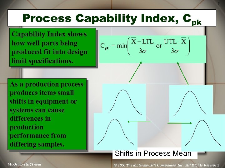
6 Process Capability Index, Cpk Capability Index shows how well parts being produced fit into design limit specifications. As a production process produces items small shifts in equipment or systems can cause differences in production performance from differing samples. Shifts in Process Mean Mc. Graw-Hill/Irwin © 2006 The Mc. Graw-Hill Companies, Inc. , All Rights Reserved.
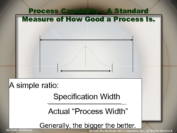
7 Process Capability – A Standard Measure of How Good a Process Is. A simple ratio: Specification Width _____________________________ Actual “Process Width” Mc. Graw-Hill/Irwin Generally, the bigger the better. © 2006 The Mc. Graw-Hill Companies, Inc. , All Rights Reserved.
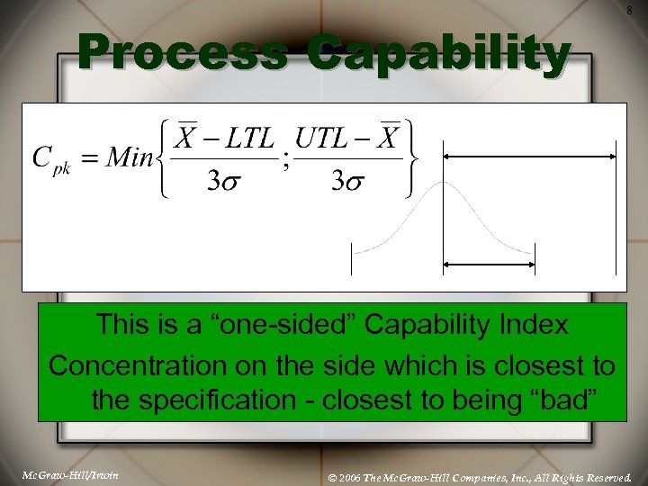
Process Capability 8 This is a “one-sided” Capability Index Concentration on the side which is closest to the specification - closest to being “bad” Mc. Graw-Hill/Irwin © 2006 The Mc. Graw-Hill Companies, Inc. , All Rights Reserved.
The Cereal Box Example 9 We are the maker of this cereal. Consumer Reports has just published an article that shows that we frequently have less than 15 ounces of cereal in a box. Let’s assume that the government says that we must be within ± 5 percent of the weight advertised on the box. Upper Tolerance Limit = 16 +. 05(16) = 16. 8 ounces Lower Tolerance Limit = 16 –. 05(16) = 15. 2 ounces We go out and buy 1, 000 boxes of cereal and find that they weight an average of 15. 875 ounces with a standard deviation of. 529 ounces. Mc. Graw-Hill/Irwin © 2006 The Mc. Graw-Hill Companies, Inc. , All Rights Reserved.
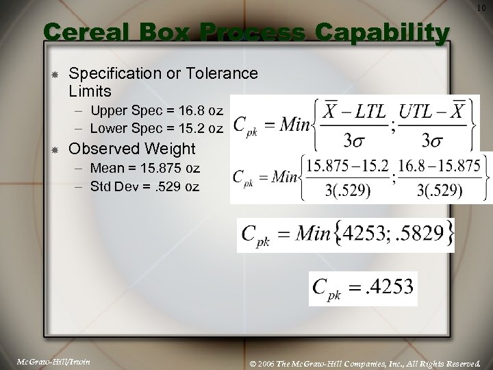
10 Cereal Box Process Capability Specification or Tolerance Limits – Upper Spec = 16. 8 oz – Lower Spec = 15. 2 oz Observed Weight – Mean = 15. 875 oz – Std Dev =. 529 oz Mc. Graw-Hill/Irwin © 2006 The Mc. Graw-Hill Companies, Inc. , All Rights Reserved.
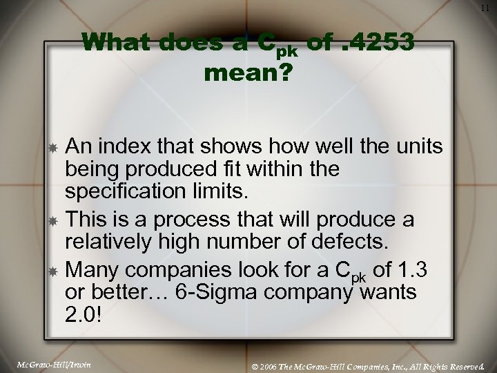
11 What does a Cpk of. 4253 mean? An index that shows how well the units being produced fit within the specification limits. This is a process that will produce a relatively high number of defects. Many companies look for a Cpk of 1. 3 or better… 6 -Sigma company wants 2. 0! Mc. Graw-Hill/Irwin © 2006 The Mc. Graw-Hill Companies, Inc. , All Rights Reserved.
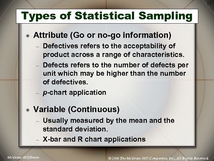
12 Types of Statistical Sampling Attribute (Go or no-go information) – – – Defectives refers to the acceptability of product across a range of characteristics. Defects refers to the number of defects per unit which may be higher than the number of defectives. p-chart application Variable (Continuous) – – Mc. Graw-Hill/Irwin Usually measured by the mean and the standard deviation. X-bar and R chart applications © 2006 The Mc. Graw-Hill Companies, Inc. , All Rights Reserved.
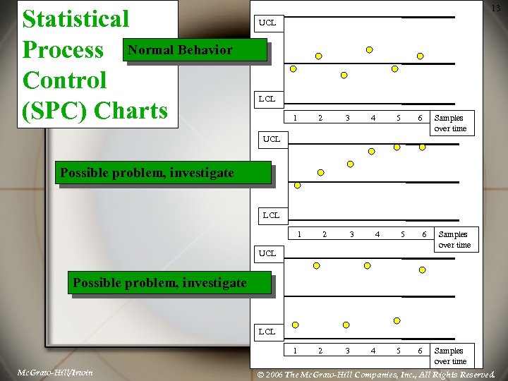
Statistical Process Normal Behavior Control (SPC) Charts 13 UCL LCL 1 2 3 4 5 6 Samples over time UCL Possible problem, investigate LCL 1 2 3 4 5 6 UCL Samples over time Possible problem, investigate LCL 1 Mc. Graw-Hill/Irwin 2 3 4 5 6 Samples over time © 2006 The Mc. Graw-Hill Companies, Inc. , All Rights Reserved.
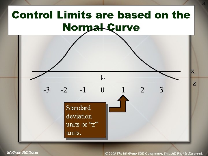
14 Control Limits are based on the Normal Curve m -3 -2 -1 0 1 2 3 x z Standard deviation units or “z” units. Mc. Graw-Hill/Irwin © 2006 The Mc. Graw-Hill Companies, Inc. , All Rights Reserved.
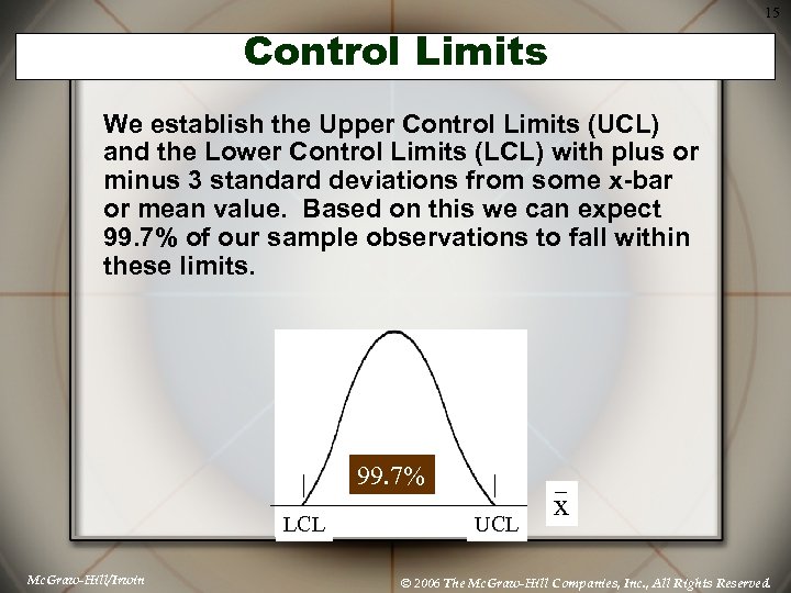
15 Control Limits We establish the Upper Control Limits (UCL) and the Lower Control Limits (LCL) with plus or minus 3 standard deviations from some x-bar or mean value. Based on this we can expect 99. 7% of our sample observations to fall within these limits. 99. 7% LCL Mc. Graw-Hill/Irwin UCL x © 2006 The Mc. Graw-Hill Companies, Inc. , All Rights Reserved.
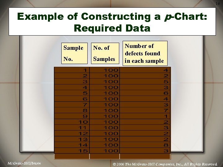
16 Example of Constructing a p-Chart: Required Data Sample No. Mc. Graw-Hill/Irwin No. of Samples Number of defects found in each sample © 2006 The Mc. Graw-Hill Companies, Inc. , All Rights Reserved.
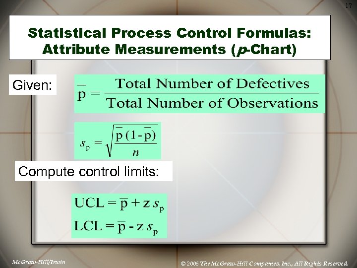
17 Statistical Process Control Formulas: Attribute Measurements (p-Chart) Given: Compute control limits: Mc. Graw-Hill/Irwin © 2006 The Mc. Graw-Hill Companies, Inc. , All Rights Reserved.
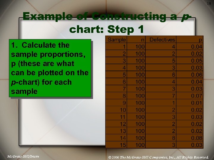
18 Example of Constructing a pchart: Step 1 1. Calculate the sample proportions, p (these are what can be plotted on the p-chart) for each sample Mc. Graw-Hill/Irwin © 2006 The Mc. Graw-Hill Companies, Inc. , All Rights Reserved.
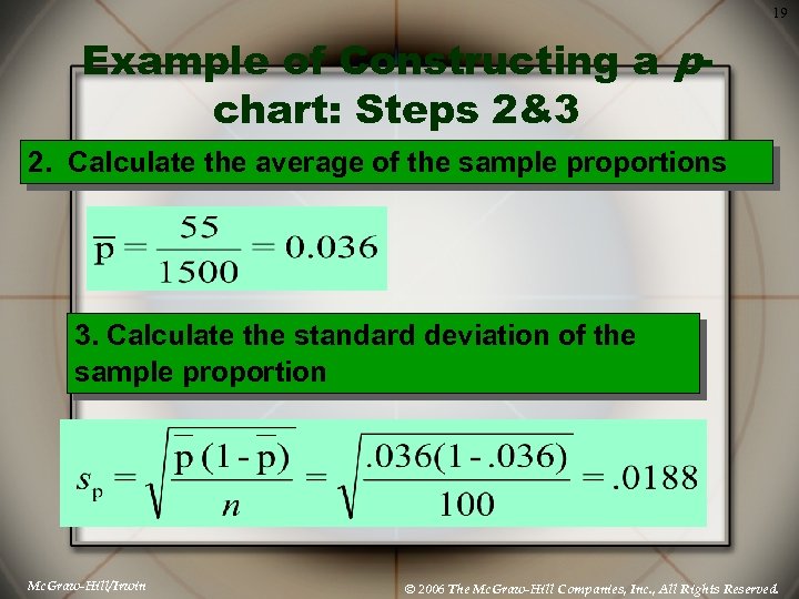
19 Example of Constructing a pchart: Steps 2&3 2. Calculate the average of the sample proportions 3. Calculate the standard deviation of the sample proportion Mc. Graw-Hill/Irwin © 2006 The Mc. Graw-Hill Companies, Inc. , All Rights Reserved.
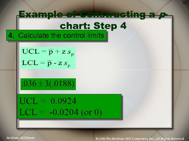
20 Example of Constructing a pchart: Step 4 4. Calculate the control limits UCL = 0. 0924 LCL = -0. 0204 (or 0) Mc. Graw-Hill/Irwin © 2006 The Mc. Graw-Hill Companies, Inc. , All Rights Reserved.
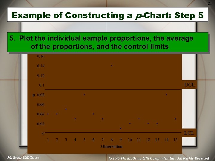
21 Example of Constructing a p-Chart: Step 5 5. Plot the individual sample proportions, the average of the proportions, and the control limits UCL LCL Mc. Graw-Hill/Irwin © 2006 The Mc. Graw-Hill Companies, Inc. , All Rights Reserved.
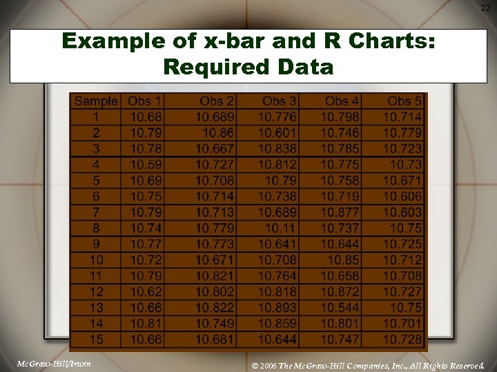
22 Example of x-bar and R Charts: Required Data Mc. Graw-Hill/Irwin © 2006 The Mc. Graw-Hill Companies, Inc. , All Rights Reserved.
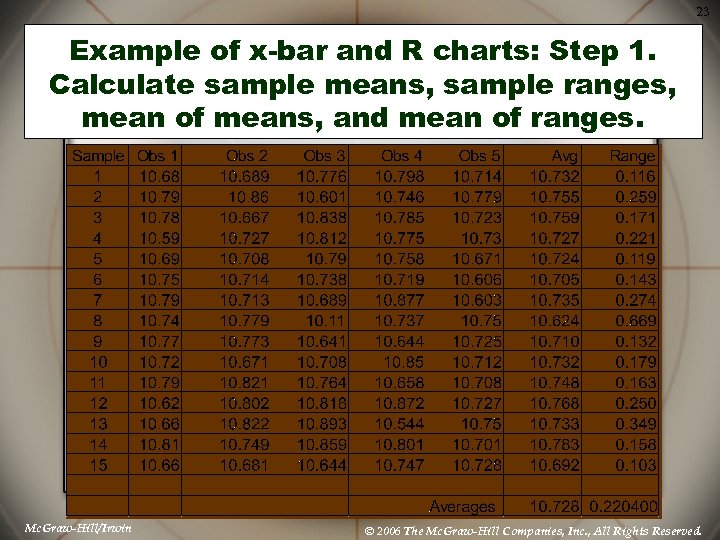
23 Example of x-bar and R charts: Step 1. Calculate sample means, sample ranges, mean of means, and mean of ranges. Mc. Graw-Hill/Irwin © 2006 The Mc. Graw-Hill Companies, Inc. , All Rights Reserved.
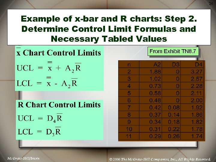
24 Example of x-bar and R charts: Step 2. Determine Control Limit Formulas and Necessary Tabled Values From Exhibit TN 8. 7 Mc. Graw-Hill/Irwin © 2006 The Mc. Graw-Hill Companies, Inc. , All Rights Reserved.
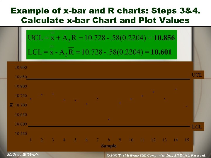
Example of x-bar and R charts: Steps 3&4. Calculate x-bar Chart and Plot Values 25 UCL LCL Mc. Graw-Hill/Irwin © 2006 The Mc. Graw-Hill Companies, Inc. , All Rights Reserved.
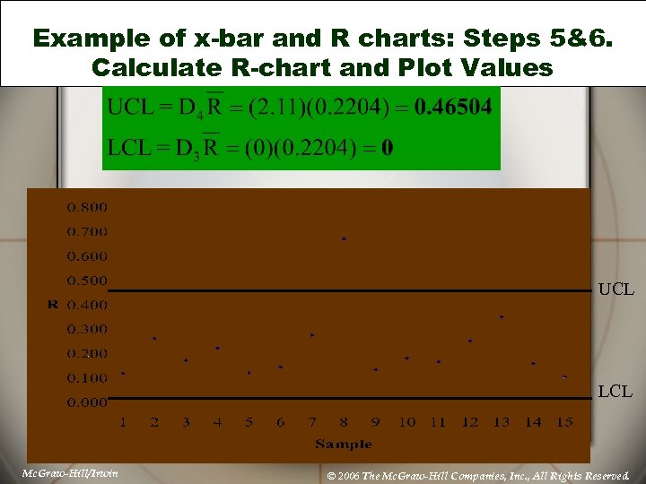
26 Example of x-bar and R charts: Steps 5&6. Calculate R-chart and Plot Values UCL LCL Mc. Graw-Hill/Irwin © 2006 The Mc. Graw-Hill Companies, Inc. , All Rights Reserved.
27 Basic Forms of Statistical Sampling for Quality Control Acceptance Sampling is sampling to accept or reject the immediate lot of product at hand Statistical Process Control is sampling to determine if the process is within acceptable limits Mc. Graw-Hill/Irwin © 2006 The Mc. Graw-Hill Companies, Inc. , All Rights Reserved.
28 Acceptance Sampling Purposes – – Determine quality level Ensure quality is within predetermined level Advantages – – – Mc. Graw-Hill/Irwin Economy Less handling damage Fewer inspectors Upgrading of the inspection job Applicability to destructive testing Entire lot rejection (motivation for improvement) © 2006 The Mc. Graw-Hill Companies, Inc. , All Rights Reserved.
29 Acceptance Sampling (Continued) Disadvantages – – – Risks of accepting “bad” lots and rejecting “good” lots Added planning and documentation Sample provides less information than 100 -percent inspection Mc. Graw-Hill/Irwin © 2006 The Mc. Graw-Hill Companies, Inc. , All Rights Reserved.
30 Acceptance Sampling: Single Sampling Plan A simple goal Determine (1) how many units, n, to sample from a lot, and (2) the maximum number of defective items, c, that can be found in the sample before the lot is rejected Mc. Graw-Hill/Irwin © 2006 The Mc. Graw-Hill Companies, Inc. , All Rights Reserved.
31 Risk Acceptable Quality Level (AQL) – The a (Producer’s risk) – The probability of rejecting a good lot Lot Tolerance Percent Defective (LTPD) – Max. acceptable percentage of defectives defined by producer Percentage of defectives that defines consumer’s rejection point The (Consumer’s risk) – The probability of accepting a bad lot Mc. Graw-Hill/Irwin © 2006 The Mc. Graw-Hill Companies, Inc. , All Rights Reserved.
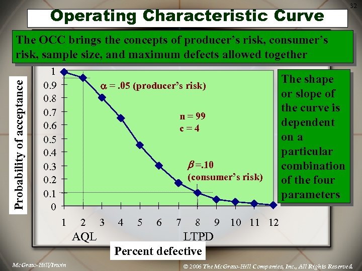
Operating Characteristic Curve 32 Probability of acceptance The OCC brings the concepts of producer’s risk, consumer’s risk, sample size, and maximum defects allowed together 1 0. 9 0. 8 0. 7 0. 6 0. 5 0. 4 0. 3 0. 2 0. 1 0 a =. 05 (producer’s risk) n = 99 c=4 =. 10 (consumer’s risk) 1 2 AQL Mc. Graw-Hill/Irwin 3 4 5 6 7 8 9 The shape or slope of the curve is dependent on a particular combination of the four parameters 10 11 12 LTPD Percent defective © 2006 The Mc. Graw-Hill Companies, Inc. , All Rights Reserved.
33 Example: Acceptance Sampling Problem Zypercom, a manufacturer of video interfaces, purchases printed wiring boards from an outside vender, Procard has set an acceptable quality level of 1% and accepts a 5% risk of rejecting lots at or below this level. Zypercom considers lots with 3% defectives to be unacceptable and will assume a 10% risk of accepting a defective lot. Develop a sampling plan for Zypercom and determine a rule to be followed by the receiving inspection personnel. Mc. Graw-Hill/Irwin © 2006 The Mc. Graw-Hill Companies, Inc. , All Rights Reserved.
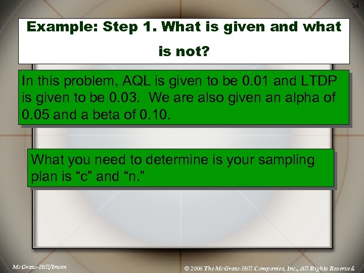
34 Example: Step 1. What is given and what is not? In this problem, AQL is given to be 0. 01 and LTDP is given to be 0. 03. We are also given an alpha of 0. 05 and a beta of 0. 10. What you need to determine is your sampling plan is “c” and “n. ” Mc. Graw-Hill/Irwin © 2006 The Mc. Graw-Hill Companies, Inc. , All Rights Reserved.
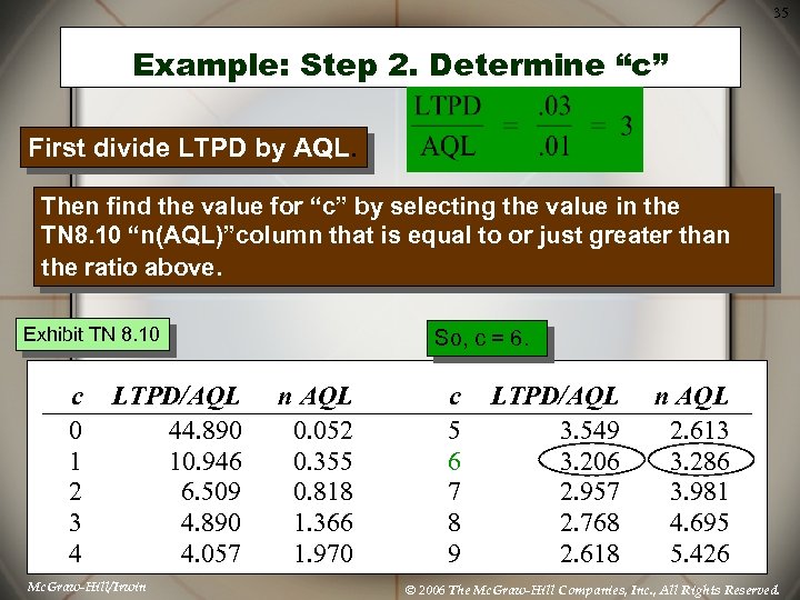
35 Example: Step 2. Determine “c” First divide LTPD by AQL. Then find the value for “c” by selecting the value in the TN 8. 10 “n(AQL)”column that is equal to or just greater than the ratio above. Exhibit TN 8. 10 c 0 1 2 3 4 LTPD/AQL 44. 890 10. 946 6. 509 4. 890 4. 057 Mc. Graw-Hill/Irwin So, c = 6. n AQL 0. 052 0. 355 0. 818 1. 366 1. 970 c 5 6 7 8 9 LTPD/AQL 3. 549 3. 206 2. 957 2. 768 2. 618 n AQL 2. 613 3. 286 3. 981 4. 695 5. 426 © 2006 The Mc. Graw-Hill Companies, Inc. , All Rights Reserved.
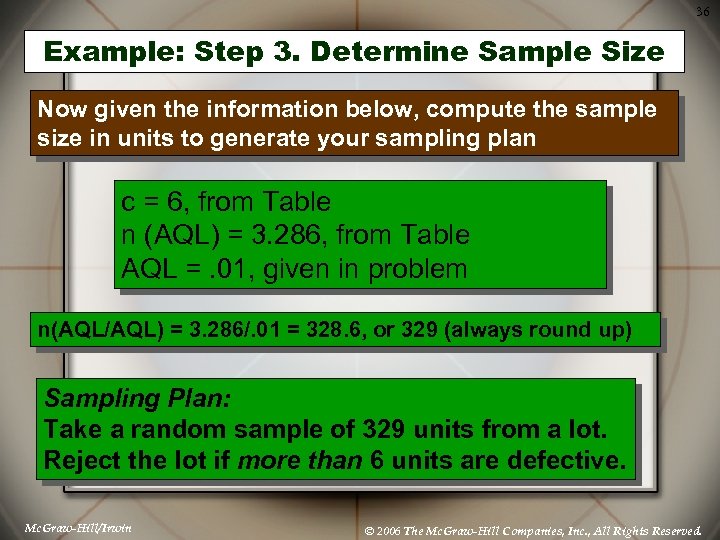
36 Example: Step 3. Determine Sample Size Now given the information below, compute the sample size in units to generate your sampling plan c = 6, from Table n (AQL) = 3. 286, from Table AQL =. 01, given in problem n(AQL/AQL) = 3. 286/. 01 = 328. 6, or 329 (always round up) Sampling Plan: Take a random sample of 329 units from a lot. Reject the lot if more than 6 units are defective. Mc. Graw-Hill/Irwin © 2006 The Mc. Graw-Hill Companies, Inc. , All Rights Reserved.
6c9413d5283a48b504a47e4db39cb14d.ppt