1 Performance Space Modeling for Hierarchical Synthesis

1

Performance Space Modeling for Hierarchical Synthesis of Analog Integrated Circuits Georges Gielen, Trent Mc. Conaghy, Tom Eeckelaert ESAT-MICAS, Katholieke Universiteit Leuven, Belgium DAC, June 2005, Anaheim 2

Outline • introduction : hierarchical design • performance estimation • design space organization and traversal • conclusions 3

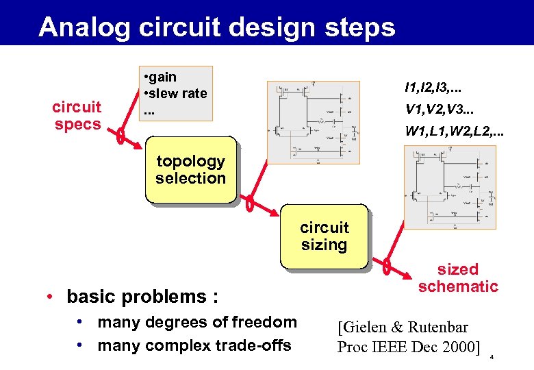Analog circuit design steps circuit specs • gain • slew rate. . . I 1, I 2, I 3, . . . V 1, V 2, V 3. . . W 1, L 1, W 2, L 2, . . . topology selection circuit sizing • basic problems : • many degrees of freedom • many complex trade-offs sized schematic [Gielen & Rutenbar Proc IEEE Dec 2000] 4

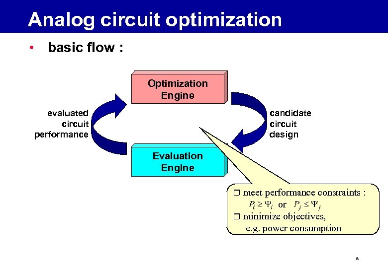Analog circuit optimization • basic flow : Optimization Engine evaluated circuit performance candidate circuit design Evaluation Engine meet performance constraints : or r minimize objectives, e. g. power consumption r 5

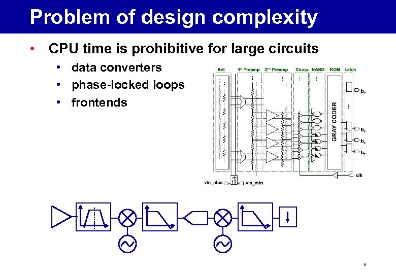Problem of design complexity • CPU time is prohibitive for large circuits • data converters • phase-locked loops • frontends 6

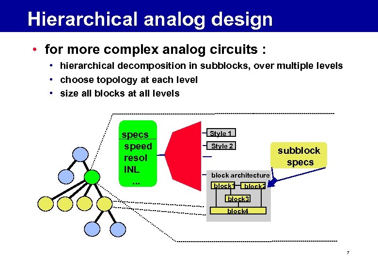Hierarchical analog design refinement • for more complex analog circuits : • hierarchical decomposition in subblocks, over multiple levels • choose topology at each level • size all blocks at all levels specs speed resol INL. . . Style 1 Style 2 subblock specs block architecture block 1 block 2 block 3 block 4 7

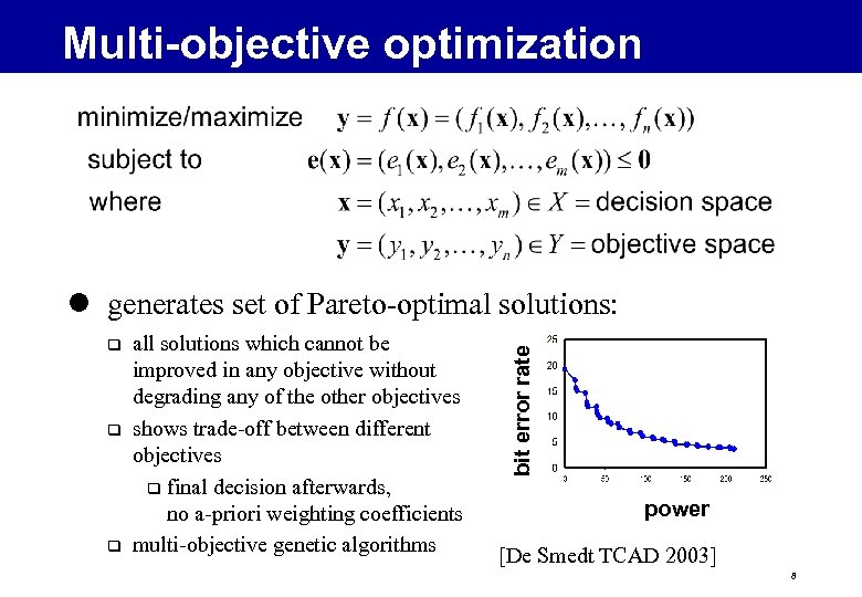Multi-objective optimization q q q all solutions which cannot be improved in any objective without degrading any of the other objectives shows trade-off between different objectives q final decision afterwards, no a-priori weighting coefficients multi-objective genetic algorithms bit error rate l generates set of Pareto-optimal solutions: power [De Smedt TCAD 2003] 8

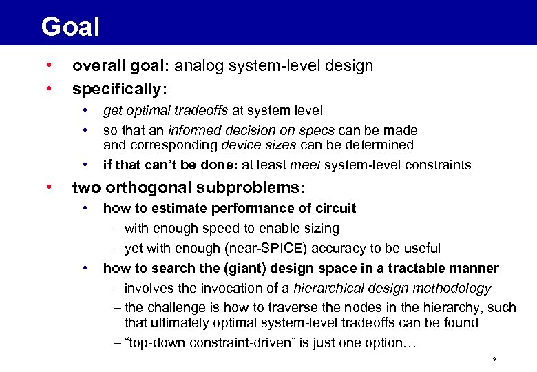Goal • • overall goal: analog system-level design specifically: • • get optimal tradeoffs at system level so that an informed decision on specs can be made and corresponding device sizes can be determined if that can’t be done: at least meet system-level constraints two orthogonal subproblems: • • how to estimate performance of circuit – with enough speed to enable sizing – yet with enough (near-SPICE) accuracy to be useful how to search the (giant) design space in a tractable manner – involves the invocation of a hierarchical design methodology – the challenge is how to traverse the nodes in the hierarchy, such that ultimately optimal system-level tradeoffs can be found – “top-down constraint-driven” is just one option… 9

Outline • introduction : hierarchical design • performance estimation – goals – dynamic modeling and subsets – static modeling and subsets • design space organization and traversal • conclusions 10

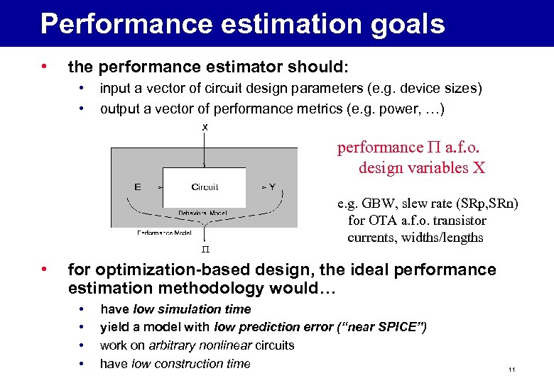Performance estimation goals • the performance estimator should: • • input a vector of circuit design parameters (e. g. device sizes) output a vector of performance metrics (e. g. power, …) performance P a. f. o. design variables X e. g. GBW, slew rate (SRp, SRn) for OTA a. f. o. transistor currents, widths/lengths • for optimization-based design, the ideal performance estimation methodology would… • • have low simulation time yield a model with low prediction error (“near SPICE”) work on arbitrary nonlinear circuits have low construction time 11

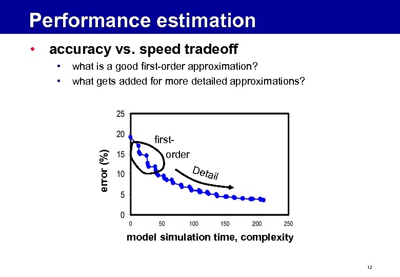Performance estimation • accuracy vs. speed tradeoff what is a good first-order approximation? what gets added for more detailed approximations? error (%) • • firstorder Deta il model simulation time, complexity 12

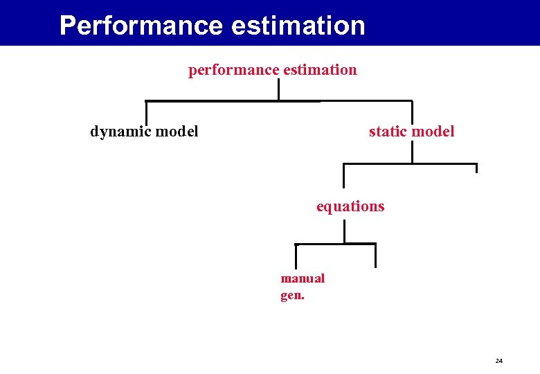
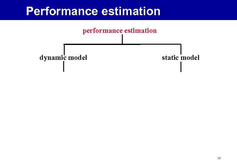Performance estimation performance estimation dynamic model static model 13

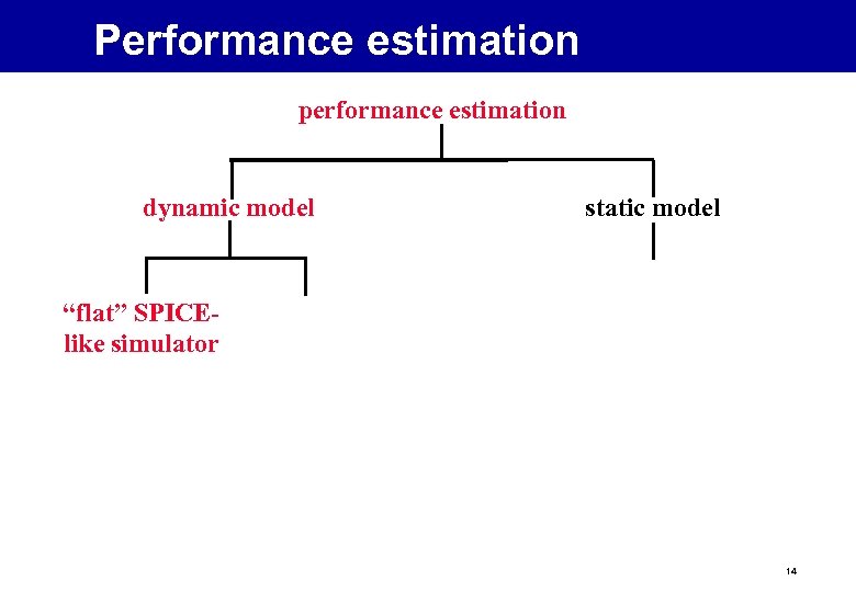Performance estimation performance estimation dynamic model static model “flat” SPICElike simulator 14

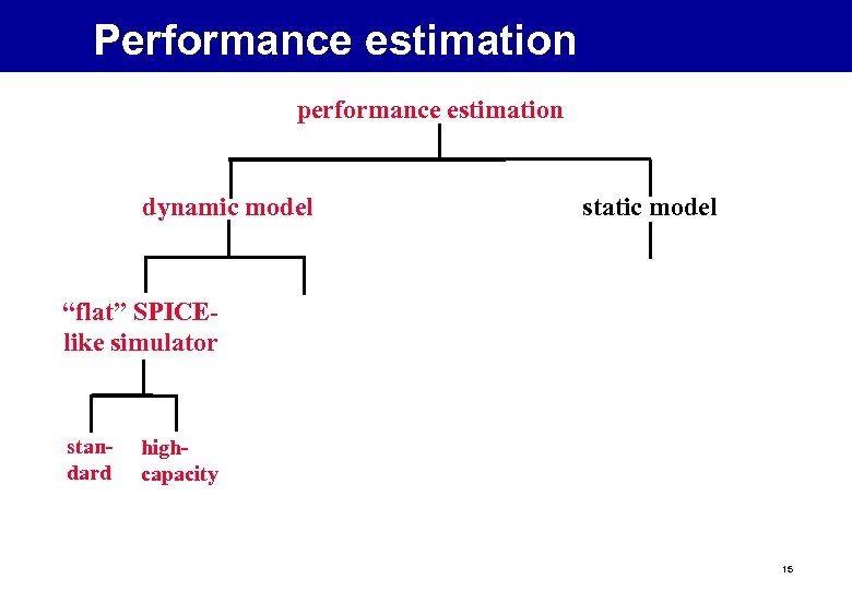Performance estimation performance estimation dynamic model static model “flat” SPICElike simulator standard highcapacity 15

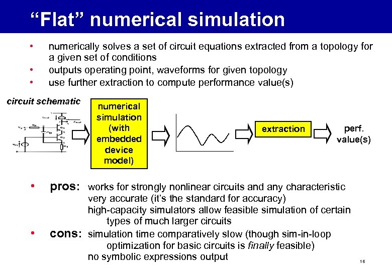“Flat” numerical simulation • • • numerically solves a set of circuit equations extracted from a topology for a given set of conditions outputs operating point, waveforms for given topology use further extraction to compute performance value(s) circuit schematic • • numerical simulation (with embedded device model) extraction perf. value(s) pros: works for strongly nonlinear circuits and any characteristic cons: very accurate (it’s the standard for accuracy) high-capacity simulators allow feasible simulation of certain types of much larger circuits simulation time comparatively slow (though sim-in-loop optimization for basic circuits is finally feasible) no symbolic expressions output 16

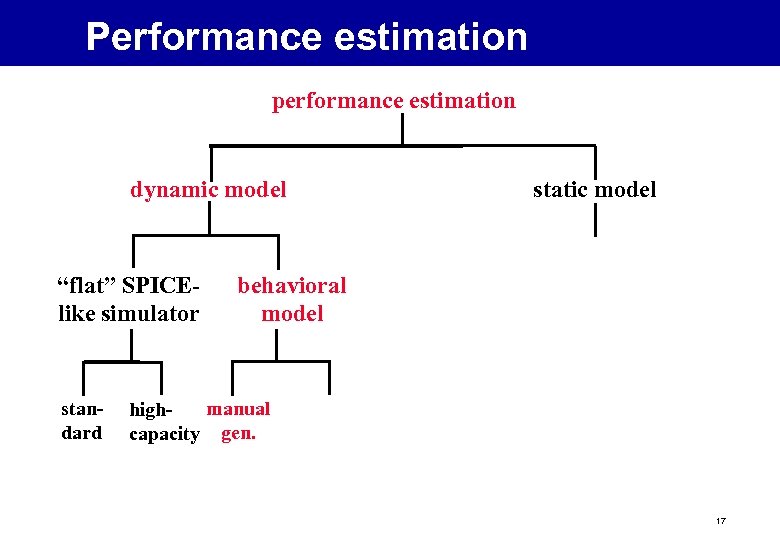Performance estimation performance estimation dynamic model “flat” SPICElike simulator standard static model behavioral model manual highcapacity gen. 17

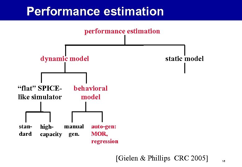Performance estimation performance estimation dynamic model “flat” SPICElike simulator standard static model behavioral model manual highcapacity gen. auto-gen: MOR, regression [Gielen & Phillips CRC 2005] 18

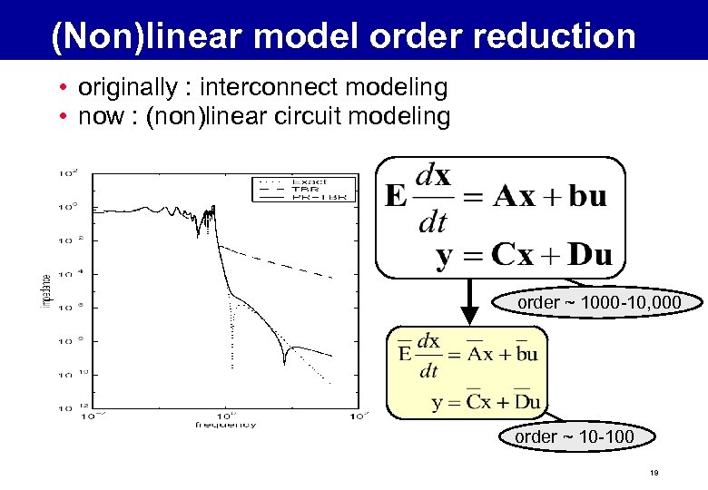(Non)linear model order reduction • originally : interconnect modeling • now : (non)linear circuit modeling order ~ 1000 -10, 000 order ~ 10 -100 19

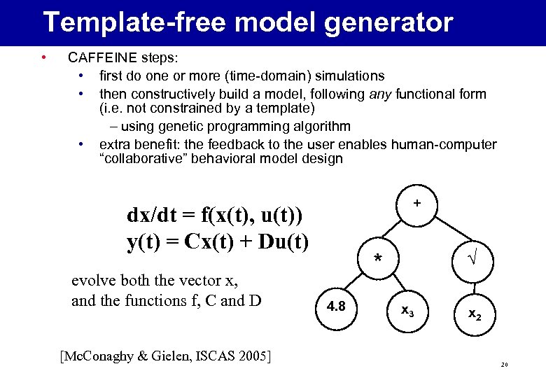Template-free model generator • CAFFEINE steps: • first do one or more (time-domain) simulations • then constructively build a model, following any functional form (i. e. not constrained by a template) – using genetic programming algorithm • extra benefit: the feedback to the user enables human-computer “collaborative” behavioral model design + dx/dt = f(x(t), u(t)) y(t) = Cx(t) + Du(t) evolve both the vector x, and the functions f, C and D [Mc. Conaghy & Gielen, ISCAS 2005] √ * 4. 8 x 3 x 2 20

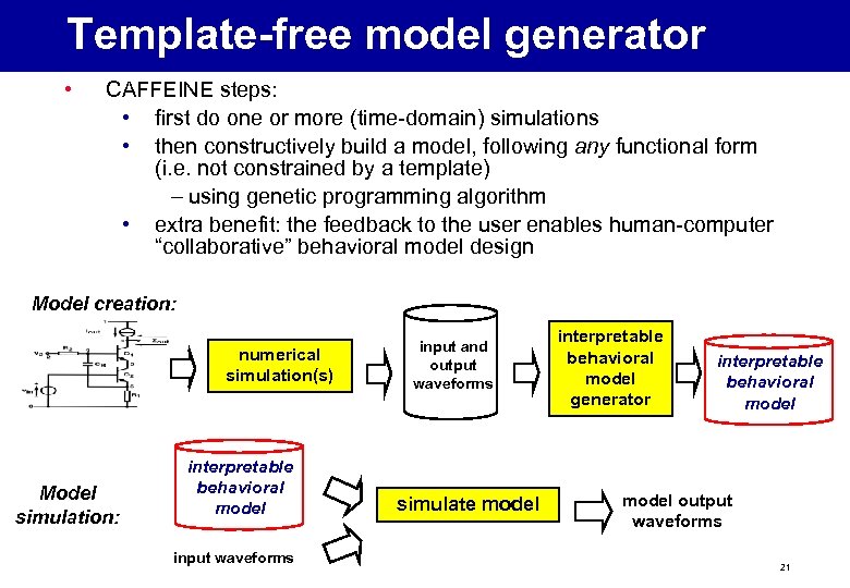Template-free model generator • CAFFEINE steps: • first do one or more (time-domain) simulations • then constructively build a model, following any functional form (i. e. not constrained by a template) – using genetic programming algorithm • extra benefit: the feedback to the user enables human-computer “collaborative” behavioral model design Model creation: numerical simulation(s) Model simulation: interpretable behavioral model input waveforms input and output waveforms simulate model interpretable behavioral model generator interpretable behavioral model output waveforms 21

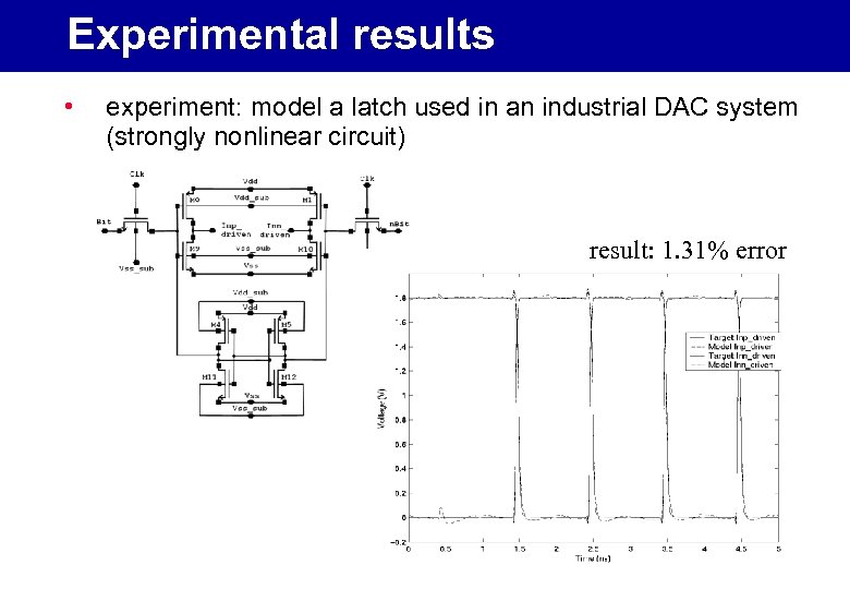Experimental results • experiment: model a latch used in an industrial DAC system (strongly nonlinear circuit) result: 1. 31% error 22

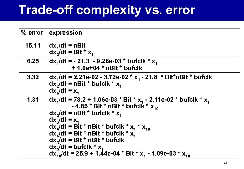Trade-off complexity vs. error % error 15. 11 6. 25 3. 32 1. 31 expression dx 1/dt = n. Bit dx 2/dt = Bit * x 1 dx 1/dt = - 21. 3 - 9. 28 e-03 * bufclk * x 1 + 1. 0 e+04 * n. Bit * bufclk dx 1/dt = 2. 21 e-02 - 3. 72 e-02 * x 1 - 21. 8 * Bit*n. Bit * bufclk dx 2/dt = n. Bit * bufclk * x 1 dx 6/dt = x 1 dx 1/dt = 78. 2 + 1. 06 e-03 * Bit * x 1 - 2. 11 e-02 * bufclk * x 1 - 4. 85 * Bit * n. Bit * bufclk * x 10 dx 2/dt = n. Bit * bufclk * x 1 dx 3/dt = x 1 dx 4/dt = Bit * n. Bit * bufclk * x 10 dx 6/dt = Bit * n. Bit * bufclk * x 1 dx 8/dt = Bit * n. Bit * bufclk dx 9/dt = bufclk * x 1 dx 10/dt = 25. 9 + 1. 44 e-04 * Bit * x 1 - 1. 89 e-03 * x 10 23

Performance estimation performance estimation dynamic model static model equations manual gen. 24

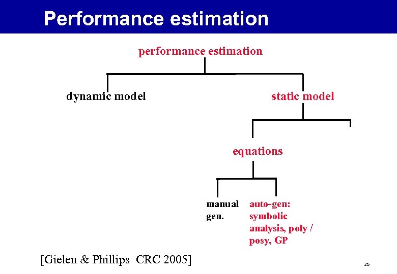Performance estimation performance estimation dynamic model static model equations manual gen. [Gielen & Phillips CRC 2005] auto-gen: symbolic analysis, poly / posy, GP 25

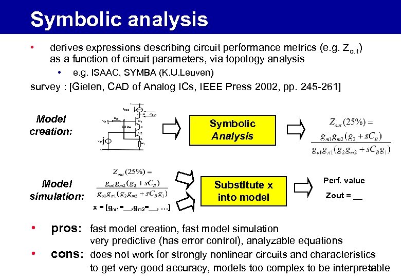Symbolic analysis • derives expressions describing circuit performance metrics (e. g. Zout) as a function of circuit parameters, via topology analysis • e. g. ISAAC, SYMBA (K. U. Leuven) survey : [Gielen, CAD of Analog ICs, IEEE Press 2002, pp. 245 -261] Model creation: Symbolic Analysis Model simulation: Substitute x into model Perf. value Zout = __ x = [gm 1=__, gm 2=__, …] • • pros: fast model creation, fast model simulation cons: very predictive (has error control), analyzable equations does not work for strongly nonlinear circuits and characteristics 26 to get very good accuracy, models too complex to be interpretable

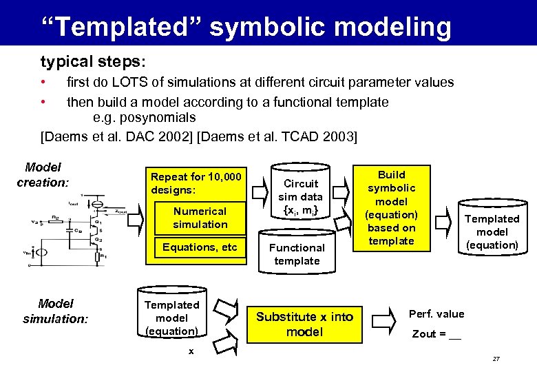“Templated” symbolic modeling typical steps: • • first do LOTS of simulations at different circuit parameter values then build a model according to a functional template e. g. posynomials [Daems et al. DAC 2002] [Daems et al. TCAD 2003] Model creation: Repeat for 10, 000 designs: Numerical simulation Equations, etc Model simulation: Templated model (equation) x Circuit sim data {xi, mi} Functional template Substitute x into model Build symbolic model (equation) based on template Templated model (equation) Perf. value Zout = __ 27

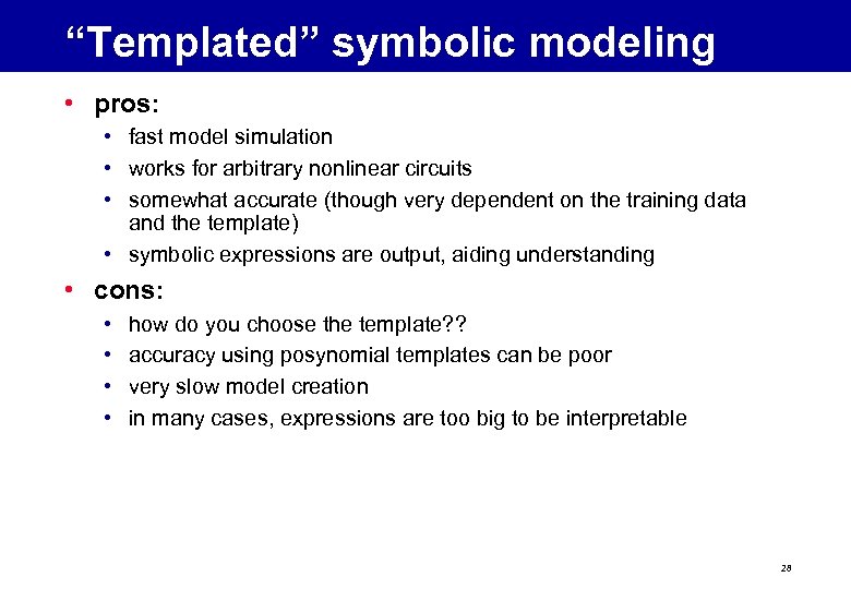“Templated” symbolic modeling • pros: • fast model simulation • works for arbitrary nonlinear circuits • somewhat accurate (though very dependent on the training data and the template) • symbolic expressions are output, aiding understanding • cons: • • how do you choose the template? ? accuracy using posynomial templates can be poor very slow model creation in many cases, expressions are too big to be interpretable 28

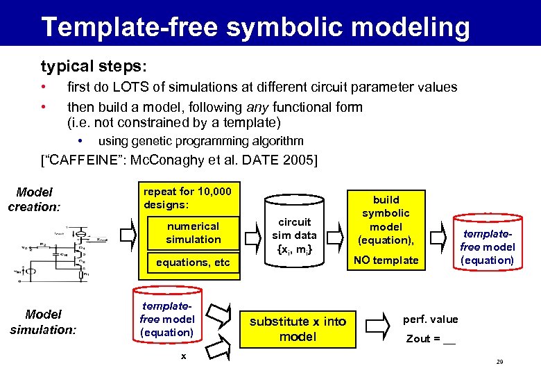Template-free symbolic modeling typical steps: • • first do LOTS of simulations at different circuit parameter values then build a model, following any functional form (i. e. not constrained by a template) • using genetic programming algorithm [“CAFFEINE”: Mc. Conaghy et al. DATE 2005] Model creation: repeat for 10, 000 designs: numerical simulation equations, etc Model simulation: templatefree model (equation) x circuit sim data {xi, mi} substitute x into model build symbolic model (equation), NO templatefree model (equation) perf. value Zout = __ 29

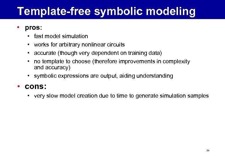Template-free symbolic modeling • pros: • • fast model simulation works for arbitrary nonlinear circuits accurate (though very dependent on training data) no template to choose (therefore improvements in complexity and accuracy) • symbolic expressions are output, aiding understanding • cons: • very slow model creation due to time to generate simulation samples 30

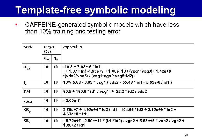Template-free symbolic modeling • CAFFEINE-generated symbolic models which have less than 10% training and testing error perf. target (%) expression qwc qtc ALF 10 10 -10. 3 + 7. 08 e-5 / id 1 + 1. 87 * ln( -1. 95 e+9 + 1. 00 e+10 / (vsg 1*vsg 3)+ 1. 42 e+9 *(vds 2*vsd 5) / (vsg 1*vgs 2*vsg 5*id 2)) fu 10 10 10^( 5. 68 - 0. 03 * vsg 1 / vds 2 - 55. 43 * id 1+ 5. 63 e-6 / id 1 ) PM 10 10 90. 5 + 190. 6 * id 1 / vsg 1 + 22. 2 * id 2 / vds 2 voffset 10 10 - 2. 00 e-3 SRp 10 10 2. 36 e+7 + 1. 95 e+4 * id 2 / id 1 - 104. 69 / id 2 + 2. 15 e+9 * id 2 + 4. 63 e+8 * id 1 SRn 10 10 - 5. 72 e+7 - 2. 50 e+11 * (id 1*id 2) / vgs 2 + 5. 53 e+6 * vds 2 / vgs 2 + 109. 72 / id 1 31

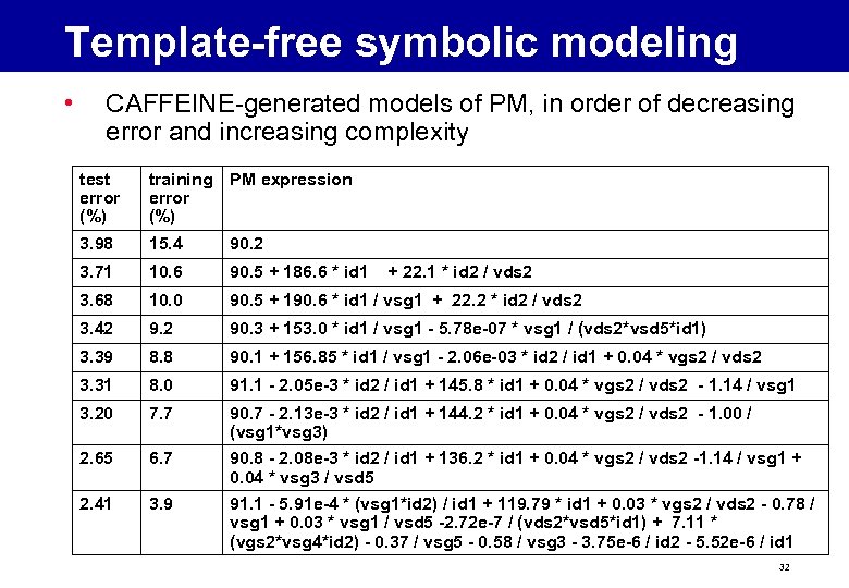Template-free symbolic modeling • CAFFEINE-generated models of PM, in order of decreasing error and increasing complexity test error (%) training PM expression error (%) 3. 98 15. 4 90. 2 3. 71 10. 6 90. 5 + 186. 6 * id 1 3. 68 10. 0 90. 5 + 190. 6 * id 1 / vsg 1 + 22. 2 * id 2 / vds 2 3. 42 9. 2 90. 3 + 153. 0 * id 1 / vsg 1 - 5. 78 e-07 * vsg 1 / (vds 2*vsd 5*id 1) 3. 39 8. 8 90. 1 + 156. 85 * id 1 / vsg 1 - 2. 06 e-03 * id 2 / id 1 + 0. 04 * vgs 2 / vds 2 3. 31 8. 0 91. 1 - 2. 05 e-3 * id 2 / id 1 + 145. 8 * id 1 + 0. 04 * vgs 2 / vds 2 - 1. 14 / vsg 1 3. 20 7. 7 90. 7 - 2. 13 e-3 * id 2 / id 1 + 144. 2 * id 1 + 0. 04 * vgs 2 / vds 2 - 1. 00 / (vsg 1*vsg 3) 2. 65 6. 7 90. 8 - 2. 08 e-3 * id 2 / id 1 + 136. 2 * id 1 + 0. 04 * vgs 2 / vds 2 -1. 14 / vsg 1 + 0. 04 * vsg 3 / vsd 5 2. 41 3. 9 91. 1 - 5. 91 e-4 * (vsg 1*id 2) / id 1 + 119. 79 * id 1 + 0. 03 * vgs 2 / vds 2 - 0. 78 / vsg 1 + 0. 03 * vsg 1 / vsd 5 -2. 72 e-7 / (vds 2*vsd 5*id 1) + 7. 11 * (vgs 2*vsg 4*id 2) - 0. 37 / vsg 5 - 0. 58 / vsg 3 - 3. 75 e-6 / id 2 - 5. 52 e-6 / id 1 + 22. 1 * id 2 / vds 2 32

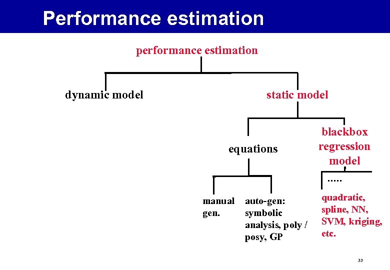Performance estimation performance estimation dynamic model static model equations manual gen. auto-gen: symbolic analysis, poly / posy, GP blackbox regression model quadratic, spline, NN, SVM, kriging, etc. 33

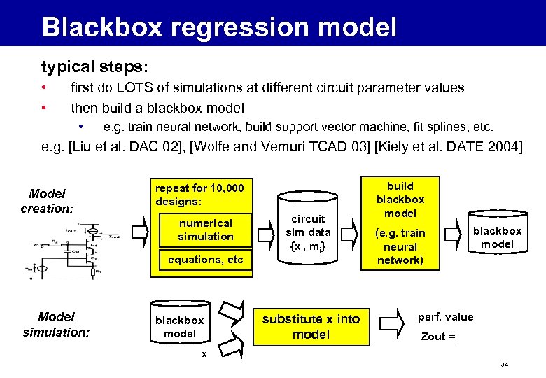Blackbox regression model typical steps: • • first do LOTS of simulations at different circuit parameter values then build a blackbox model • e. g. train neural network, build support vector machine, fit splines, etc. e. g. [Liu et al. DAC 02], [Wolfe and Vemuri TCAD 03] [Kiely et al. DATE 2004] Model creation: repeat for 10, 000 designs: numerical simulation equations, etc Model simulation: blackbox model circuit sim data {xi, mi} substitute x into model build blackbox model (e. g. train neural network) blackbox model perf. value Zout = __ x 34

Blackbox regression model • pros: • works for arbitrary nonlinear circuits • fast model simulation • somewhat accurate (though very dependent on the training data!) • cons: • very slow model creation (100’s or 1000’s of simulations) • no symbolic expressions output, therefore less understanding • very hard to find one functional model that fits well everywhere – boosting between multiple models is a possible solution 35

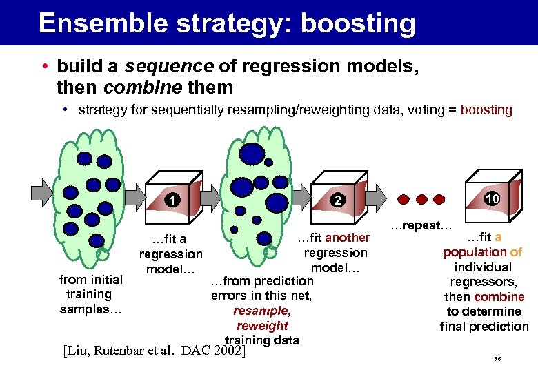Ensemble strategy: boosting • build a sequence of regression models, then combine them • strategy for sequentially resampling/reweighting data, voting = boosting 1 from initial training samples… …fit a regression model… 10 2 …fit another regression model… …from prediction errors in this net, resample, reweight training data [Liu, Rutenbar et al. DAC 2002] …repeat… …fit a population of individual regressors, then combine to determine final prediction 36

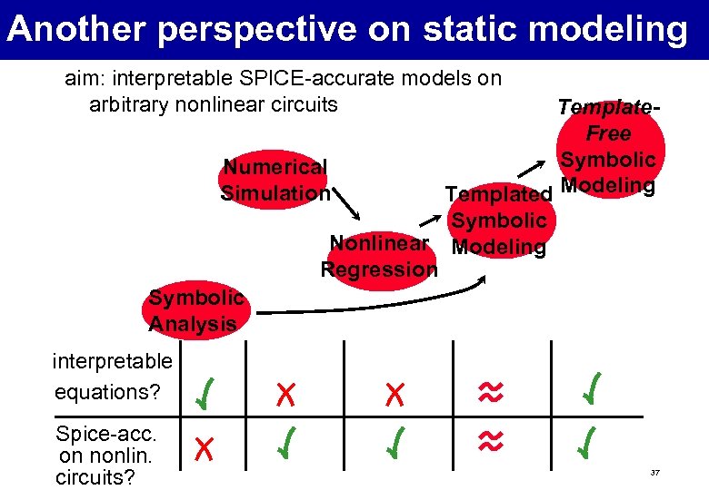Another perspective on static modeling aim: interpretable SPICE-accurate models on arbitrary nonlinear circuits Numerical Simulation Template. Free Symbolic Templated Modeling Symbolic Nonlinear Modeling Regression Symbolic Analysis interpretable equations? Spice-acc. on nonlin. circuits? 37

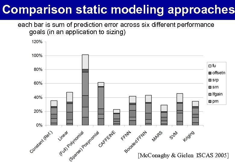Comparison static modeling approaches each bar is sum of prediction error across six different performance goals (in an application to sizing) [Mc. Conaghy & Gielen ISCAS 2005] 38

Outline • introduction : hierarchical design • performance estimation • design space organization and traversal – flat – variants of hierarchical methodologies – comparison • conclusions 39

Design space organisation & traversal design space organization & traversal 40

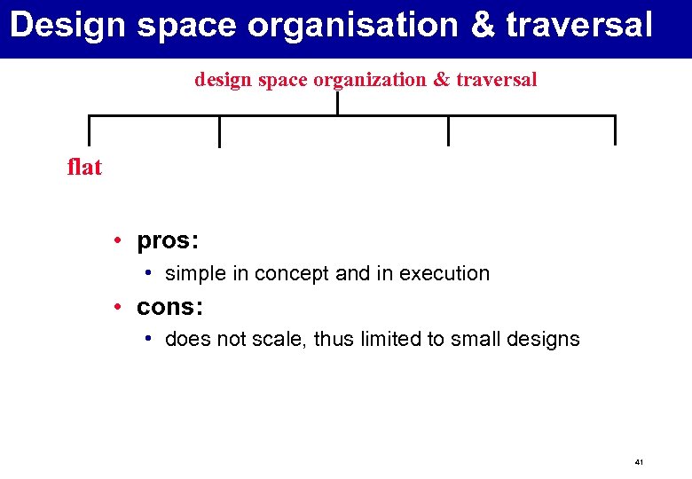Design space organisation & traversal design space organization & traversal flat • pros: • simple in concept and in execution • cons: • does not scale, thus limited to small designs 41

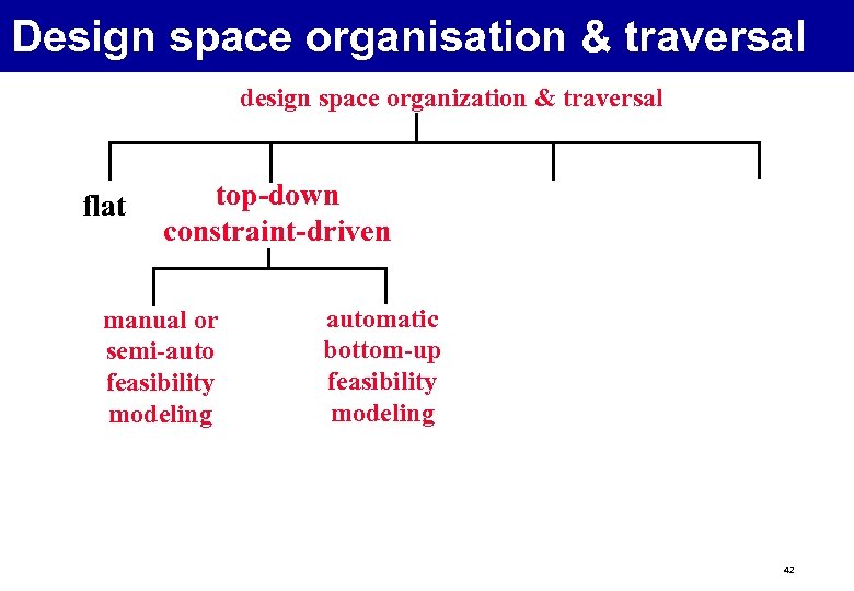Design space organisation & traversal design space organization & traversal flat top-down constraint-driven manual or semi-auto feasibility modeling automatic bottom-up feasibility modeling 42

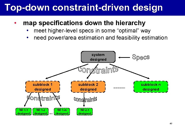Top-down constraint-driven design • map specifications down the hierarchy • meet higher-level specs in some “optimal” way • need power/area estimation and feasibility estimation system System designed subblock 1 subblock 2 Subblock 1 designed SB 1. 2 designed Subblock 2 designed SB 1. m designed subblock n Subblock n designed SB 2. 1 designed 43

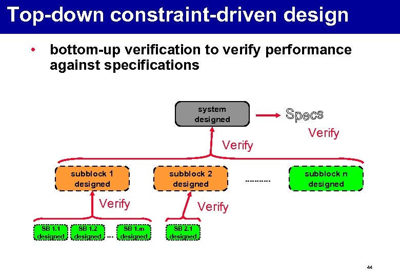Top-down constraint-driven design • bottom-up verification to verify performance against specifications system designed Verify subblock 1 designed subblock 2 designed Verify SB 1. 1 designed SB 1. 2 designed SB 1. m designed Verify subblock n designed Verify SB 2. 1 designed 44

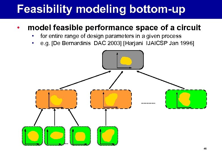Feasibility modeling bottom-up • model feasible performance space of a circuit • • for entire range of design parameters in a given process e. g. [De Bernardinis DAC 2003] [Harjani IJAICSP Jan 1996] 45

Top-down constaint-driven design • pros: • • • feasible runtime can provide system-level tradeoffs (assuming good feasibility modeling) can re-use feasibility models of building blocks the “natural choice” for advocates of top-down design cons: • • need a way to know what performance combinations of sub-blocks are feasible older feasibility modeling approaches were manual and timeconsuming, and only met constraints, not improved objectives but bottom-up feasibility modeling reconciles that – added complexity of a “model” of feasibility once feasibility modeling is done, still need to do top-down sizing steps (i. e. optimization at each hierarchical node) 46

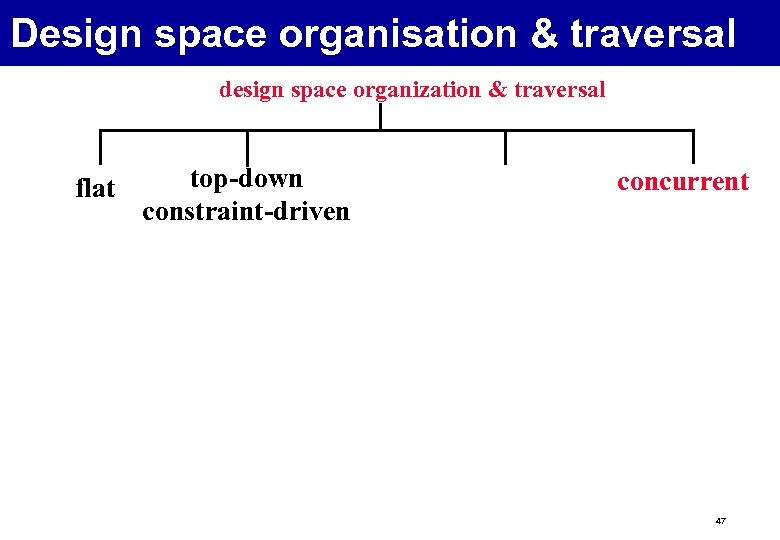Design space organisation & traversal design space organization & traversal flat top-down constraint-driven concurrent 47

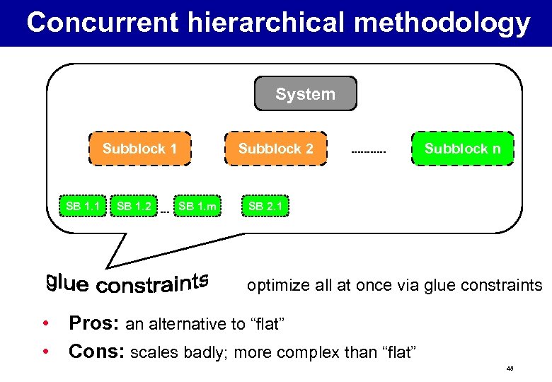Concurrent hierarchical methodology System Subblock 1 SB 1. 2 Subblock 2 SB 1. m Subblock n SB 2. 1 optimize all at once via glue constraints • Pros: an alternative to “flat” • Cons: scales badly; more complex than “flat” 48

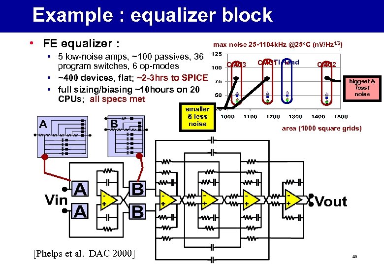Example : equalizer block • FE equalizer : max noise 25 -1104 k. Hz @25 o. C (n. V/Hz 1/2) • 5 low-noise amps, ~100 passives, 36 program switches, 6 op-modes • ~400 devices, flat; ~2 -3 hrs to SPICE • full sizing/biasing ~10 hours on 20 CPUs; all specs met smaller & less noise [Phelps et al. DAC 2000] CMU 3 TI CMU 1 Hand CMU 2 biggest & least noise area (1000 square grids) 49

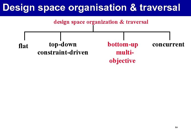Design space organisation & traversal design space organization & traversal flat top-down constraint-driven bottom-up multiobjective concurrent 50

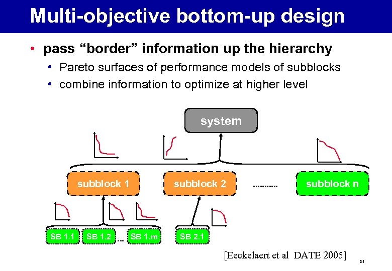Multi-objective bottom-up design • pass “border” information up the hierarchy • Pareto surfaces of performance models of subblocks • combine information to optimize at higher level system subblock 1 SB 1. 2 subblock 2 SB 1. m subblock n SB 2. 1 [Eeckelaert et al DATE 2005] 51

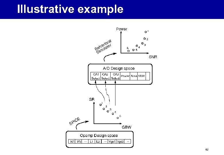Illustrative example 52

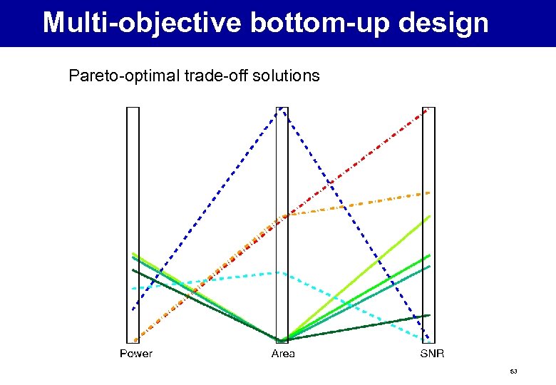Multi-objective bottom-up design Pareto-optimal trade-off solutions 53

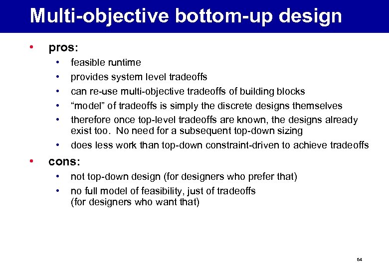Multi-objective bottom-up design • pros: • • feasible runtime provides system level tradeoffs can re-use multi-objective tradeoffs of building blocks “model” of tradeoffs is simply the discrete designs themselves therefore once top-level tradeoffs are known, the designs already exist too. No need for a subsequent top-down sizing does less work than top-down constraint-driven to achieve tradeoffs cons: • • not top-down design (for designers who prefer that) no full model of feasibility, just of tradeoffs (for designers who want that) 54

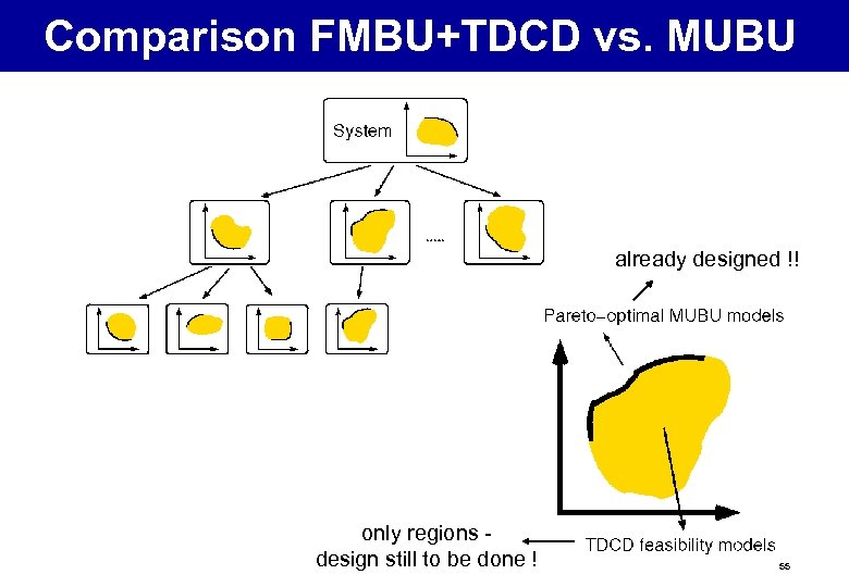Comparison FMBU+TDCD vs. MUBU already designed !! only regions design still to be done ! 55

Outline • introduction : hierarchical design • performance estimation • design space organization and traversal • conclusions 56

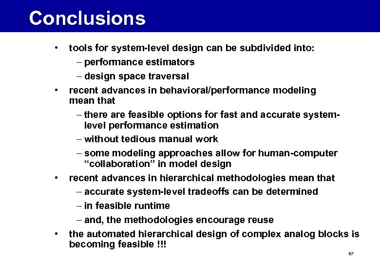Conclusions • • tools for system-level design can be subdivided into: – performance estimators – design space traversal recent advances in behavioral/performance modeling mean that – there are feasible options for fast and accurate systemlevel performance estimation – without tedious manual work – some modeling approaches allow for human-computer “collaboration” in model design recent advances in hierarchical methodologies mean that – accurate system-level tradeoffs can be determined – in feasible runtime – and, the methodologies encourage reuse the automated hierarchical design of complex analog blocks is becoming feasible !!! 57