ecd1e7c5c96a5ff7a2a918a2edb7230a.ppt
- Количество слайдов: 46
 1 of 41 Chapter 22 Adding Government and Trade to the Simple Macro Model Copyright © 2011 Pearson Canada Inc.
 2 of 41 In this chapter you will learn. . . 1. …how government purchases and tax revenues are related to national income. 2. …how exports and imports are related to national income. 3. …how to distinguish between the marginal propensity to consume and the marginal propensity to spend. 4. …why the presence of government and foreign trade reduces the value of the simple multiplier. 5. …how government can use fiscal policy to influence the level of national income. Copyright © 2011 Pearson Canada Inc.
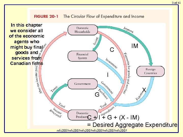 3 of 41 In this chapter we consider all of the economic agents who might buy final goods and services from Canadian firms C IM I G X C + I + G + (X - IM) = Desired Aggregate Expenditure mfc 2007 mfc 2007
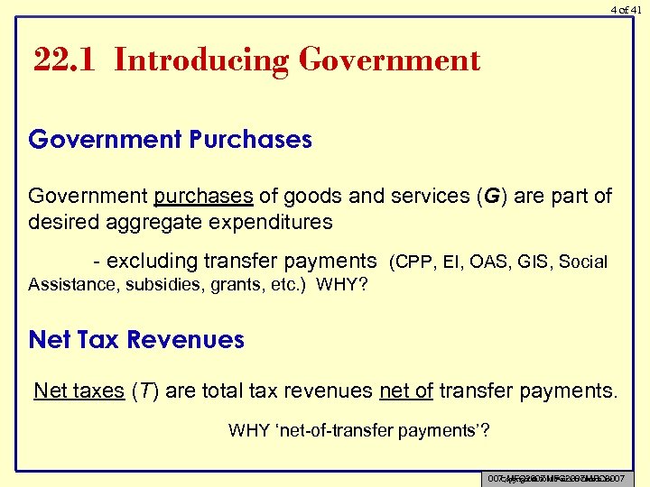 4 of 41 22. 1 Introducing Government Purchases Government purchases of goods and services (G) are part of desired aggregate expenditures - excluding transfer payments (CPP, EI, OAS, GIS, Social Assistance, subsidies, grants, etc. ) WHY? Net Tax Revenues Net taxes (T) are total tax revenues net of transfer payments. WHY ‘net-of-transfer payments’? Copyright © 2011 Pearson Canada Inc. 007, MFC 2007 MFC 2007
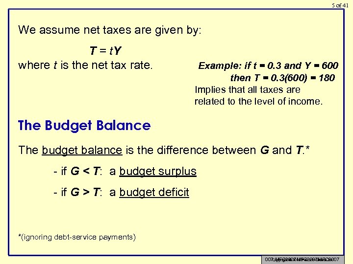 5 of 41 We assume net taxes are given by: T = t. Y where t is the net tax rate. Example: if t = 0. 3 and Y = 600 then T = 0. 3(600) = 180 Implies that all taxes are related to the level of income. The Budget Balance The budget balance is the difference between G and T. * - if G < T: a budget surplus - if G > T: a budget deficit *(ignoring debt-service payments) Copyright © 2011 Pearson Canada Inc. 007, MFC 2007 MFC 2007
 6 of 41 Provincial and Municipal Governments When measuring the overall contribution of government to desired aggregate expenditure, all levels of government must be included: - particularly important in Canada - combined purchases of provincial and municipal governments are larger than those of the federal government. Copyright © 2011 Pearson Canada Inc.
 7 of 41 Government Expenditure Function Desired government expenditure is treated as autonomous – completely unrelated to the current level of Y We write G = G Were G is determined by – what governments do! the budget process! election cycles! Mostly just the provision of ‘goods and services’ (general government, health, education, public safety, transportation, etc. ) MFC 2007, MFC 2007 MFC 2007
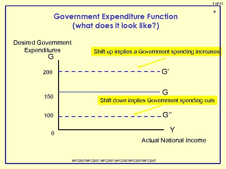 8 of 41 Government Expenditure Function (what does it look like? ) Desired Government Expenditures G Shift up implies a Government spending increases G’ 200 150 * G Shift down implies Government spending cuts G’’ 100 Y 0 Actual National Income MFC 2007, MFC 2007 MFC 2007
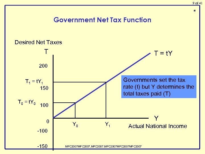 9 of 41 * Government Net Tax Function Desired Net Taxes T T = t. Y 200 Governments set the tax rate (t) but Y determines the total taxes paid (T) T 1 = t. Y 1 150 T 0 = t. Y 0 100 0 -100 -150 Y 1 Y Actual National Income MFC 2007, MFC 2007 MFC 2007
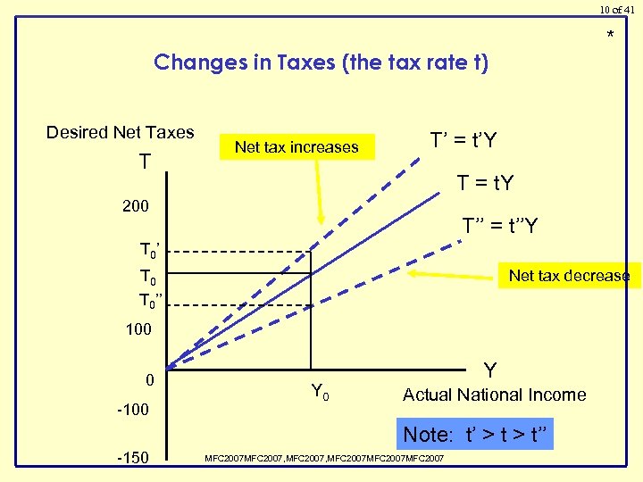 10 of 41 * Changes in Taxes (the tax rate t) Desired Net Taxes T Net tax increases T’ = t’Y T = t. Y 200 T’’ = t’’Y T 0 ’ T 0’’ Net tax decrease 100 0 -100 Y Actual National Income Note: t’ > t’’ -150 MFC 2007, MFC 2007 MFC 2007
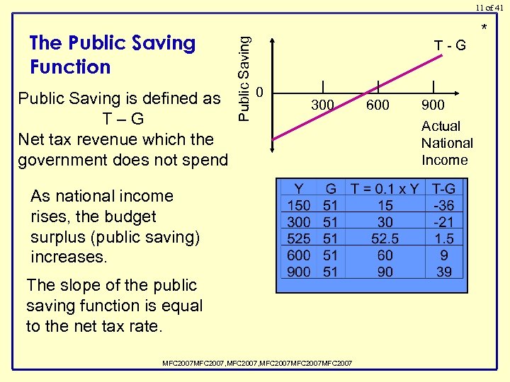 The Public Saving Function Public Saving is defined as T–G Net tax revenue which the government does not spend Public Saving 11 of 41 T-G 0 300 As national income rises, the budget surplus (public saving) increases. The slope of the public saving function is equal to the net tax rate. MFC 2007, MFC 2007 MFC 2007 600 900 Actual National Income *
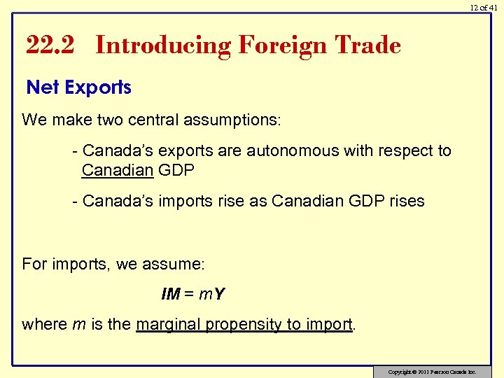 12 of 41 22. 2 Introducing Foreign Trade Net Exports We make two central assumptions: - Canada’s exports are autonomous with respect to Canadian GDP - Canada’s imports rise as Canadian GDP rises For imports, we assume: IM = m. Y where m is the marginal propensity to import. Copyright © 2011 Pearson Canada Inc.
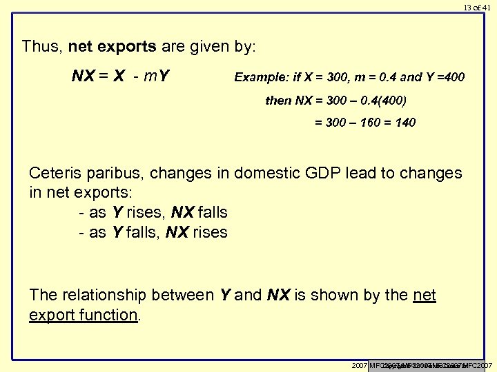 13 of 41 Thus, net exports are given by: NX = X - m. Y Example: if X = 300, m = 0. 4 and Y =400 then NX = 300 – 0. 4(400) = 300 – 160 = 140 Ceteris paribus, changes in domestic GDP lead to changes in net exports: - as Y rises, NX falls - as Y falls, NX rises The relationship between Y and NX is shown by the net export function. Copyright © 2011 Pearson Canada Inc. 2007, MFC 2007 MFC 2007
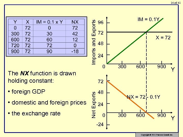 Imports and Exports 14 of 41 IM = 0. 1 Y 96 72 X = 72 48 24 0 • foreign GDP 48 600 900 Y 72 • domestic and foreign prices • the exchange rate Net Exports The NX function is drawn holding constant: 300 NX = 72 - 0. 1 Y 24 0 -24 300 600 900 Y Copyright © 2011 Pearson Canada Inc.
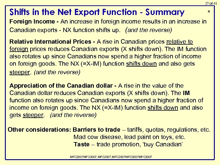
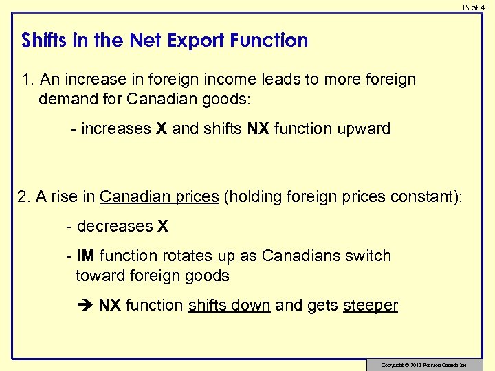 15 of 41 Shifts in the Net Export Function 1. An increase in foreign income leads to more foreign demand for Canadian goods: - increases X and shifts NX function upward 2. A rise in Canadian prices (holding foreign prices constant): - decreases X - IM function rotates up as Canadians switch toward foreign goods NX function shifts down and gets steeper Copyright © 2011 Pearson Canada Inc.
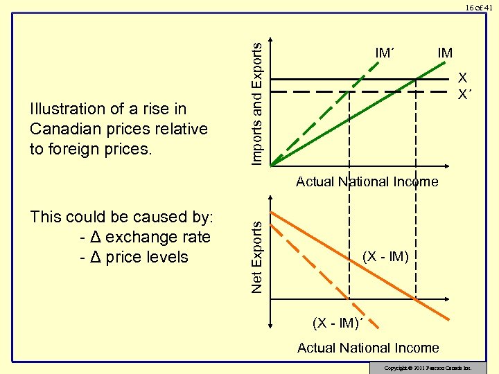 Illustration of a rise in Canadian prices relative to foreign prices. Imports and Exports 16 of 41 IM´ IM X X´ This could be caused by: - Δ exchange rate - Δ price levels Net Exports Actual National Income (X - IM)´ Actual National Income Copyright © 2011 Pearson Canada Inc.
 17 of 41 Shifts in the Net Export Function - Summary * Foreign Income - An increase in foreign income results in an increase in Canadian exports - NX function shifts up. (and the reverse) Relative International Prices - A rise in Canadian prices relative to foreign prices reduces Canadian exports (X shifts down). The IM function also rotates up since Canadians now spend a higher fraction of income on foreign goods. The NX (=X-IM) function shifts down and also gets steeper. (and the reverse) Appreciation of the Canadian dollar - A rise in the value of the Canadian dollar reduces Canadian exports (X shifts down). The IM function also rotates up since Canadians now spend a higher fraction of income on foreign goods. The NX (=X-IM) function shifts down and also gets steeper. (and the reverse) Other considerations: Barriers to trade – tariffs, quotas, regulations, etc. Mad cow disease, lead paint on toys, etc. Taste – trade promotion, ‘buy Canadian’ MFC 2007, MFC 2007 MFC 2007
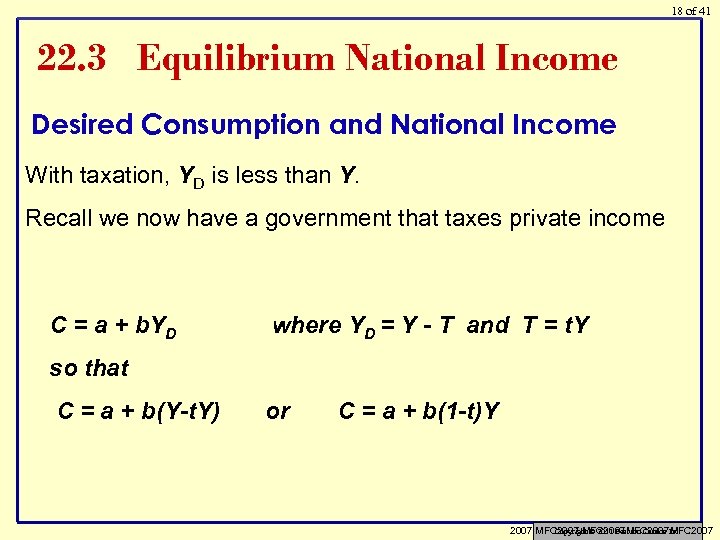 18 of 41 22. 3 Equilibrium National Income Desired Consumption and National Income With taxation, YD is less than Y. Recall we now have a government that taxes private income C = a + b. YD where YD = Y - T and T = t. Y so that C = a + b(Y-t. Y) or C = a + b(1 -t)Y Copyright © 2011 Pearson Canada Inc. 2007, MFC 2007 MFC 2007
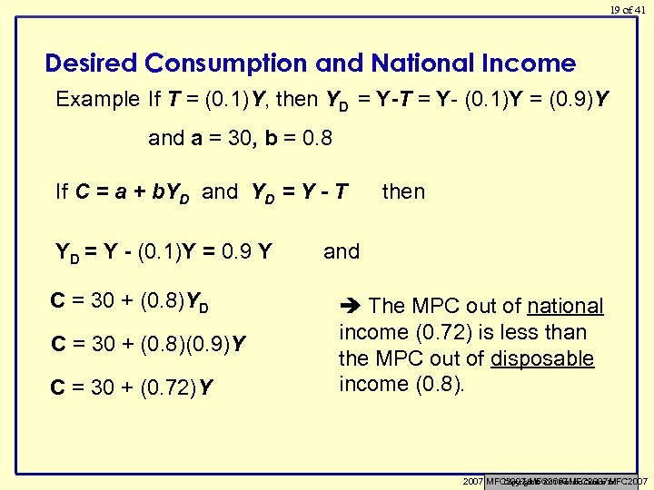 19 of 41 Desired Consumption and National Income Example If T = (0. 1)Y, then YD = Y-T = Y- (0. 1)Y = (0. 9)Y and a = 30, b = 0. 8 If C = a + b. YD and YD = Y - T YD = Y - (0. 1)Y = 0. 9 Y C = 30 + (0. 8)YD C = 30 + (0. 8)(0. 9)Y C = 30 + (0. 72)Y then and The MPC out of national income (0. 72) is less than the MPC out of disposable income (0. 8). Copyright © 2011 Pearson Canada Inc. 2007, MFC 2007 MFC 2007
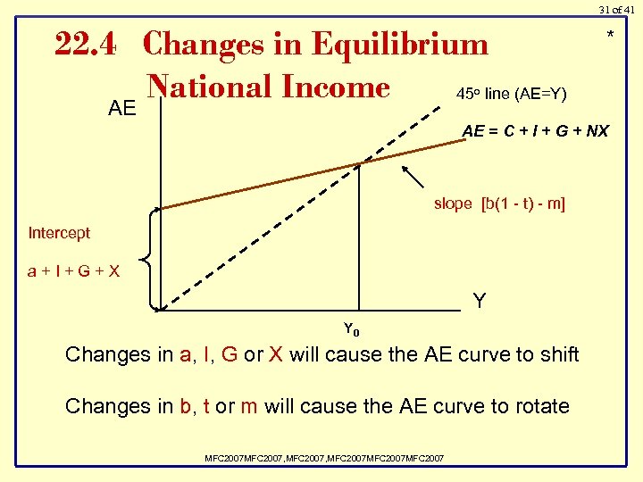
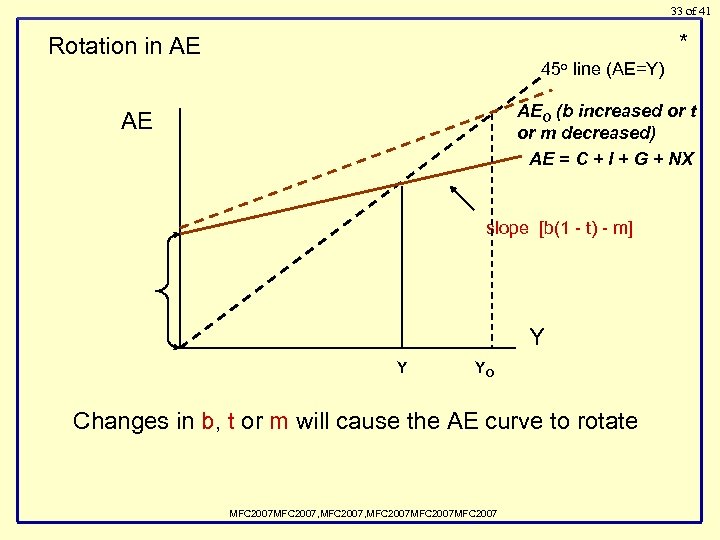
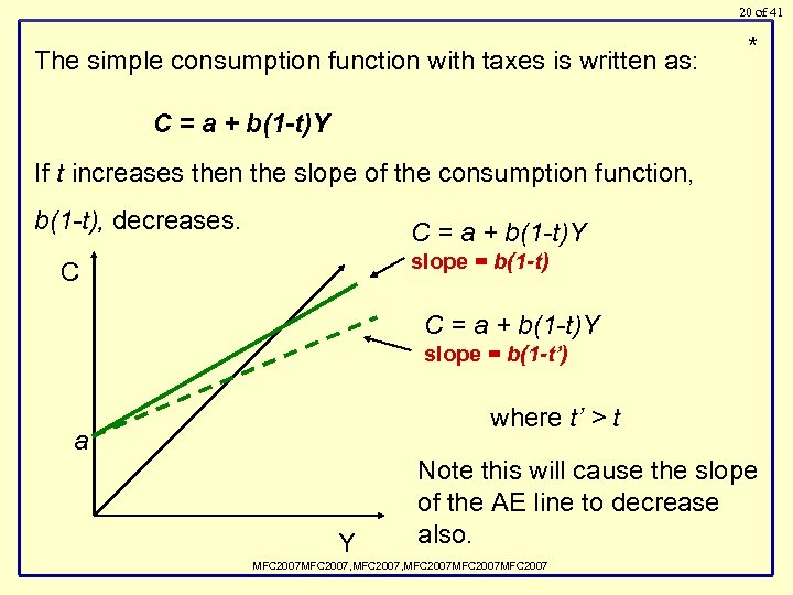 20 of 41 The simple consumption function with taxes is written as: * C = a + b(1 -t)Y If t increases then the slope of the consumption function, b(1 -t), decreases. C = a + b(1 -t)Y slope = b(1 -t) C C = a + b(1 -t)Y slope = b(1 -t’) where t’ > t a Y Note this will cause the slope of the AE line to decrease also. MFC 2007, MFC 2007 MFC 2007
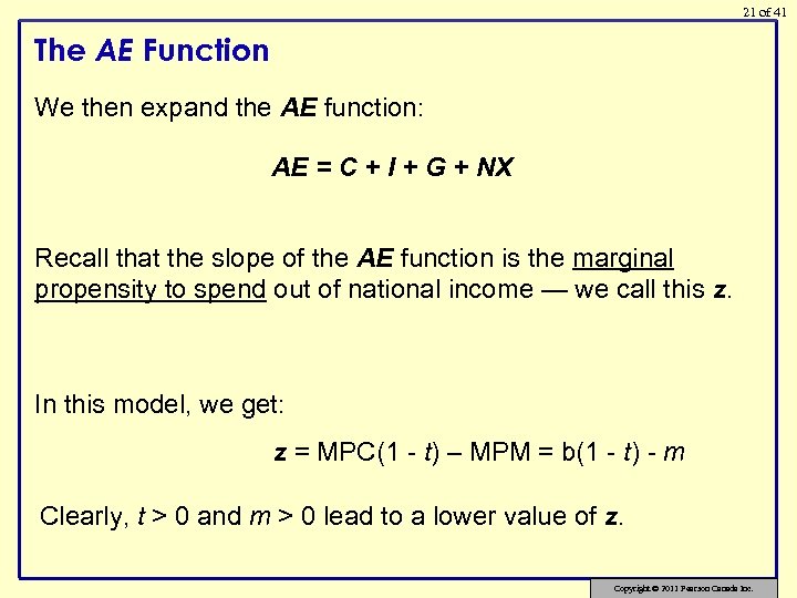 21 of 41 The AE Function We then expand the AE function: AE = C + I + G + NX Recall that the slope of the AE function is the marginal propensity to spend out of national income — we call this z. In this model, we get: z = MPC(1 - t) – MPM = b(1 - t) - m Clearly, t > 0 and m > 0 lead to a lower value of z. Copyright © 2011 Pearson Canada Inc.
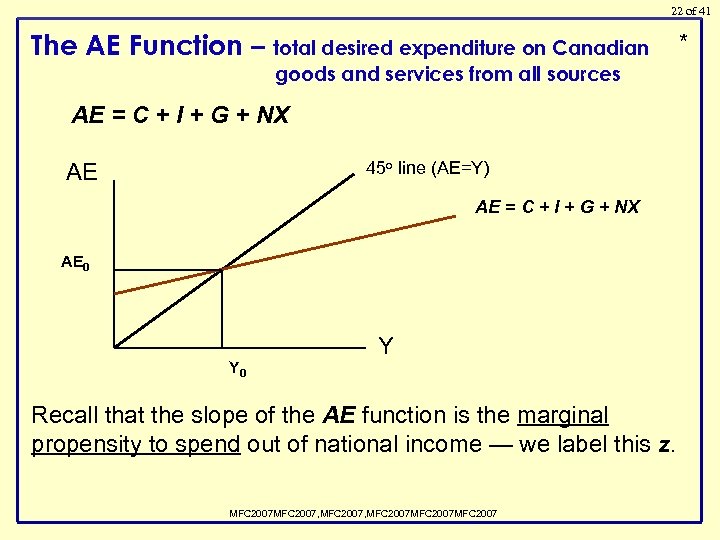 22 of 41 The AE Function – total desired expenditure on Canadian goods and services from all sources AE = C + I + G + NX 45 o line (AE=Y) AE AE = C + I + G + NX AE 0 Y Recall that the slope of the AE function is the marginal propensity to spend out of national income — we label this z. MFC 2007, MFC 2007 MFC 2007 *
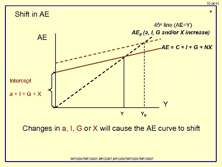
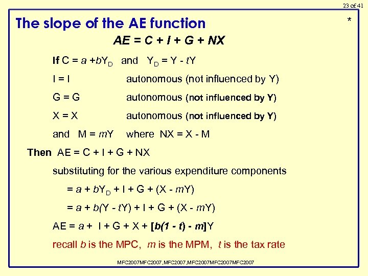 23 of 41 The slope of the AE function AE = C + I + G + NX If C = a +b. YD and YD = Y - t. Y I=I autonomous (not influenced by Y) G=G autonomous (not influenced by Y) X=X autonomous (not influenced by Y) and M = m. Y where NX = X - M Then AE = C + I + G + NX substituting for the various expenditure components = a + b. YD + I + G + (X - m. Y) = a + b(Y - t. Y) + I + G + (X - m. Y) AE = a + I + G + X + [b(1 - t) - m]Y recall b is the MPC, m is the MPM, t is the tax rate MFC 2007, MFC 2007 MFC 2007 *
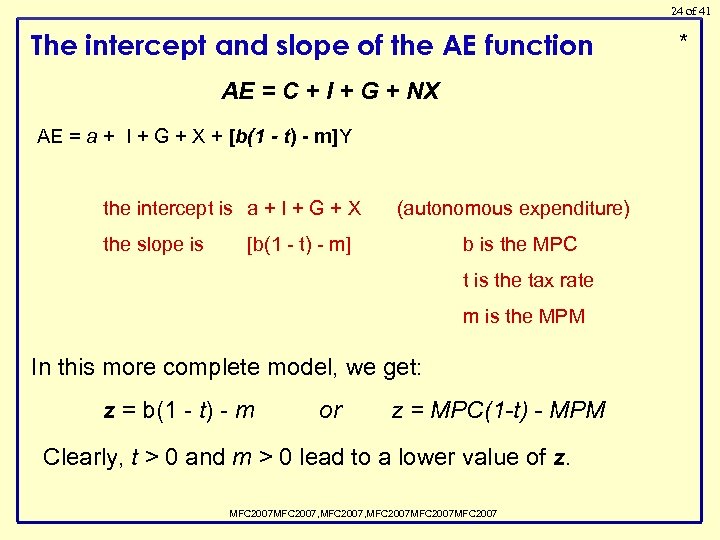 24 of 41 The intercept and slope of the AE function AE = C + I + G + NX AE = a + I + G + X + [b(1 - t) - m]Y the intercept is a + I + G + X the slope is (autonomous expenditure) [b(1 - t) - m] b is the MPC t is the tax rate m is the MPM In this more complete model, we get: z = b(1 - t) - m or z = MPC(1 -t) - MPM Clearly, t > 0 and m > 0 lead to a lower value of z. MFC 2007, MFC 2007 MFC 2007 *
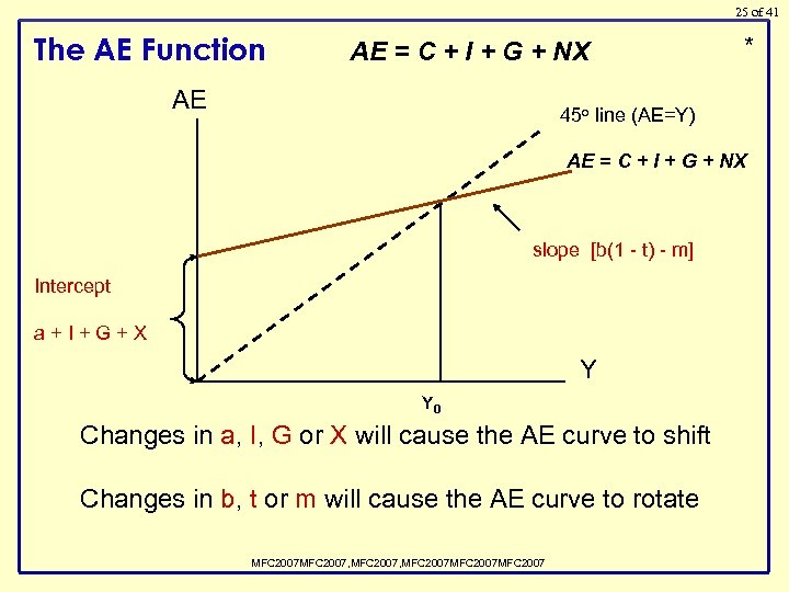 25 of 41 The AE Function AE = C + I + G + NX AE * 45 o line (AE=Y) AE = C + I + G + NX slope [b(1 - t) - m] Intercept a+I+G+X Y Y 0 Changes in a, I, G or X will cause the AE curve to shift Changes in b, t or m will cause the AE curve to rotate MFC 2007, MFC 2007 MFC 2007
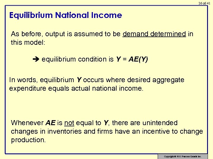 26 of 41 Equilibrium National Income As before, output is assumed to be demand determined in this model: equilibrium condition is Y = AE(Y) In words, equilibrium Y occurs where desired aggregate expenditure equals actual national income. Whenever AE is not equal to Y, there are unintended changes in inventories and firms have an incentive to change production. Copyright © 2011 Pearson Canada Inc.
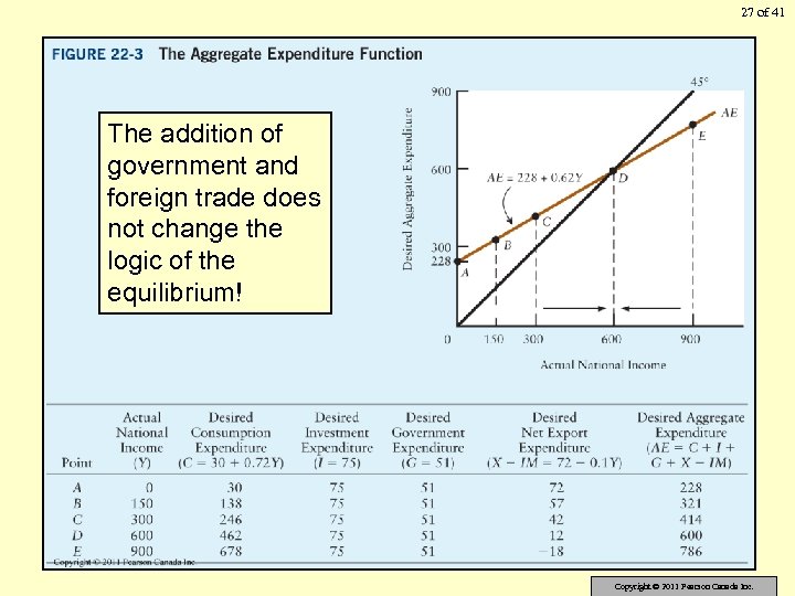 27 of 41 The addition of government and foreign trade does not change the logic of the equilibrium! Copyright © 2011 Pearson Canada Inc.
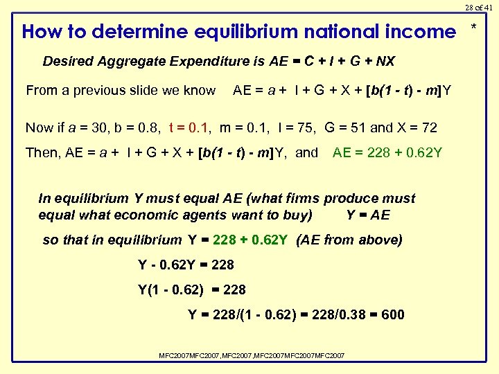 28 of 41 How to determine equilibrium national income * Desired Aggregate Expenditure is AE = C + I + G + NX From a previous slide we know AE = a + I + G + X + [b(1 - t) - m]Y Now if a = 30, b = 0. 8, t = 0. 1, m = 0. 1, I = 75, G = 51 and X = 72 Then, AE = a + I + G + X + [b(1 - t) - m]Y, and AE = 228 + 0. 62 Y In equilibrium Y must equal AE (what firms produce must equal what economic agents want to buy) Y = AE so that in equilibrium Y = 228 + 0. 62 Y (AE from above) Y - 0. 62 Y = 228 Y(1 - 0. 62) = 228 Y = 228/(1 - 0. 62) = 228/0. 38 = 600 MFC 2007, MFC 2007 MFC 2007
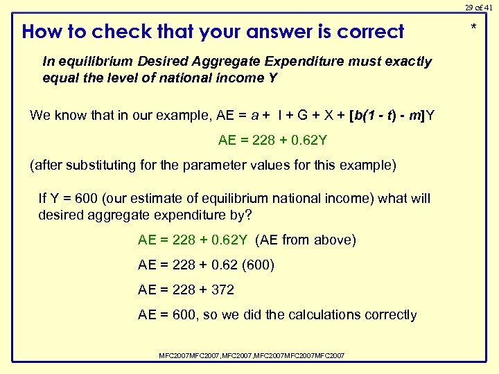 29 of 41 How to check that your answer is correct In equilibrium Desired Aggregate Expenditure must exactly equal the level of national income Y We know that in our example, AE = a + I + G + X + [b(1 - t) - m]Y AE = 228 + 0. 62 Y (after substituting for the parameter values for this example) If Y = 600 (our estimate of equilibrium national income) what will desired aggregate expenditure by? AE = 228 + 0. 62 Y (AE from above) AE = 228 + 0. 62 (600) AE = 228 + 372 AE = 600, so we did the calculations correctly MFC 2007, MFC 2007 MFC 2007 *
 30 of 41 An alternative (but equivalent) approach to determining the equilibrium level of national income is based on the relationship between national saving and the accumulation of national assets. For more details, look for The Saving-Investment Approach to Equilibrium in an Open Economy with Government in the Additional Topics section of this book’s My. Econ. Lab. www. myeconlab. com Copyright © 2011 Pearson Canada Inc.
 31 of 41 22. 4 Changes in Equilibrium National Income 45 line (AE=Y) * o AE AE = C + I + G + NX slope [b(1 - t) - m] Intercept a+I+G+X Y Y 0 Changes in a, I, G or X will cause the AE curve to shift Changes in b, t or m will cause the AE curve to rotate MFC 2007, MFC 2007 MFC 2007
 32 of 41 * Shift in AE 45 o line (AE=Y) AE 0 (a, I, G and/or X increase) AE AE = C + I + G + NX Intercept a+I+G+X Y Y Y 0 Changes in a, I, G or X will cause the AE curve to shift MFC 2007, MFC 2007 MFC 2007
 33 of 41 * Rotation in AE 45 o line (AE=Y) AEO (b increased or t or m decreased) AE = C + I + G + NX AE slope [b(1 - t) - m] Y Y YO Changes in b, t or m will cause the AE curve to rotate MFC 2007, MFC 2007 MFC 2007
 34 of 41 The Multiplier with Taxes and Imports and taxes make z smaller the simple multiplier is also smaller z = b(1 - t) - m APPLYING ECONOMIC CONCEPTS 22 -1 How Large Is Canada’s Simple Multiplier? Copyright © 2011 Pearson Canada Inc.
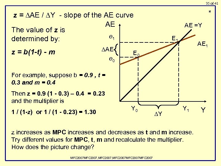 35 of 41 * z = AE / Y - slope of the AE curve AE The value of z is e 1 determined by: AE e 0 z = b(1 -t) - m AE =Y E 1 • AE 1 E 0 For example, suppose b = 0. 9 , t = 0. 3 and m = 0. 4 Then z = 0. 9 (1 - 0. 3) – 0. 4 = 0. 23 and the multiplier is 1 / (1 -z) or 1 / (1 - 0. 23) = 1. 30 Y 0 Y Y 1 z increases as MPC increases and decreases as t and m increase. Try different values for MPC, t, m and recalculate the multiplier. How does the picture change? MFC 2007, MFC 2007 MFC 2007 Y
 36 of 41 Net Exports As with other elements of AE: - if NX function shifts upward, equilibrium Y rises - if NX function shifts downward, equilibrium Y falls Exports are autonomous with respect to domestic GDP, but they depend on: - foreign income - domestic and foreign prices - exchange rate - tastes Copyright © 2011 Pearson Canada Inc.
 37 of 41 Fiscal Policy Fiscal policy is the use of the government’s spending and tax policies. Any policy that attempts to stabilize Y at or near Y* is called stabilization policy. (lots of problems with this but lets do theory anyway) It is often clear in which direction fiscal policy could be adjusted, but less clear how much is necessary. Copyright © 2011 Pearson Canada Inc.
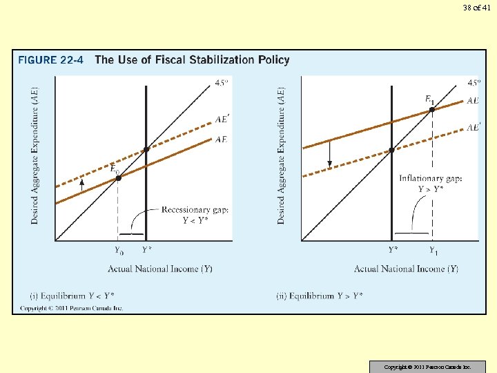 38 of 41 Copyright © 2011 Pearson Canada Inc.
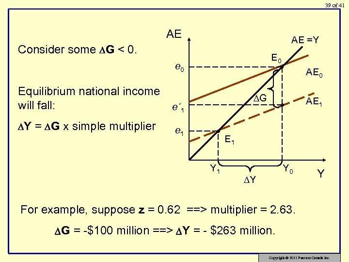 39 of 41 AE AE =Y Consider some G < 0. E 0 e 0 Equilibrium national income will fall: e´ 1 Y e 1 • = G x simple multiplier G • Y 1 • AE 0 AE 1 Y 0 Y Y For example, suppose z = 0. 62 ==> multiplier = 2. 63. G = -$100 million ==> Y = - $263 million. Copyright © 2011 Pearson Canada Inc.
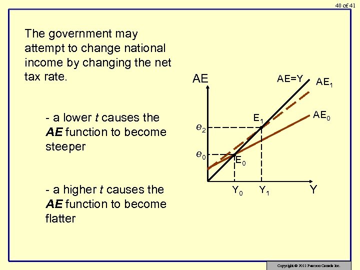 40 of 41 The government may attempt to change national income by changing the net tax rate. - a lower t causes the AE function to become steeper - a higher t causes the AE function to become flatter AE AE=Y E 1 e 2 e 0 • • E AE 1 AE 0 0 Y 1 Y Copyright © 2011 Pearson Canada Inc.
 41 of 41 Governments can also combine an increase in government purchases with an increase in tax revenues in such a way that the budget is left unchanged. How do such balanced budget changes affect the level of national income? To see more details on this type of fiscal policy, look for What is the Balanced Budget Multiplier? in the Additional Topics section of this book’s My. Econ. Lab. www. myeconlab. com Copyright © 2011 Pearson Canada Inc.
 42 of 41 22. 5 Demand-Determined Output Our simple macro model (Chapters 21 and 22) is based on three central concepts: • equilibrium national income • the simple multiplier • demand-determined output The second and third are closely connected to our assumption of a constant price level. Copyright © 2011 Pearson Canada Inc.
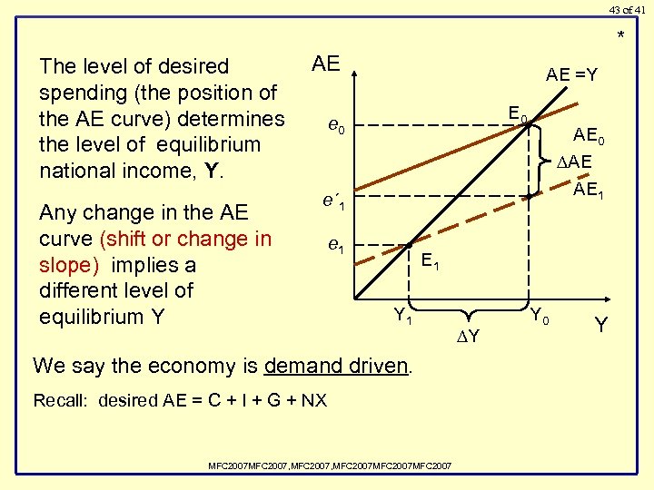 43 of 41 * The level of desired spending (the position of the AE curve) determines the level of equilibrium national income, Y. Any change in the AE curve (shift or change in slope) implies a different level of equilibrium Y AE AE =Y E 0 e 0 • • e´ 1 e 1 • AE 0 AE AE 1 Y 1 We say the economy is demand driven. Recall: desired AE = C + I + G + NX MFC 2007, MFC 2007 MFC 2007 Y Y 0 Y
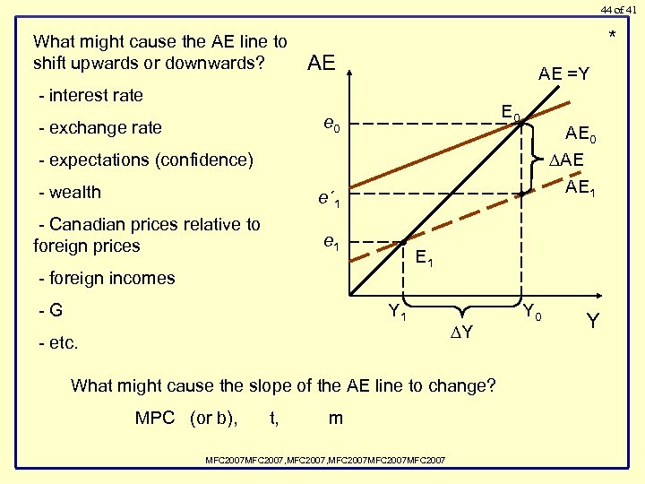 44 of 41 What might cause the AE line to shift upwards or downwards? * AE AE =Y - interest rate E 0 e 0 - exchange rate • - expectations (confidence) - wealth e´ 1 - Canadian prices relative to foreign prices e 1 • • - foreign incomes -G E 1 Y 1 - etc. Y What might cause the slope of the AE line to change? MPC (or b), t, AE 0 AE AE 1 m MFC 2007, MFC 2007 MFC 2007 Y 0 Y
 45 of 41 To this point we have assumed that firms change output and not price when the rate of production is not equal to the rate of sales. When is this a reasonable assumption? 1. When output is below potential, firms can increase output without increasing their costs. 2. When firms are price setters they often respond to shocks by changing output (and only later changing their price). In the next chapter, we allow a variable price level: - more complicated - more realistic Copyright © 2011 Pearson Canada Inc.
 46 of 41 Copyright © 2011 Pearson Canada Inc.


