1 Measures of location and dispersion Part 2

1 Measures of location and dispersion Part 2 Analysis of Variance

СHAPTER QUESTIONS Measures of Variability: Range, mean absolute deviation (MAD), Variance, Standard Deviation, Coefficient of Variation Measures of dispersion for ungrouped data Measures of dispersion for grouped data Mean and variance of the alternative feature

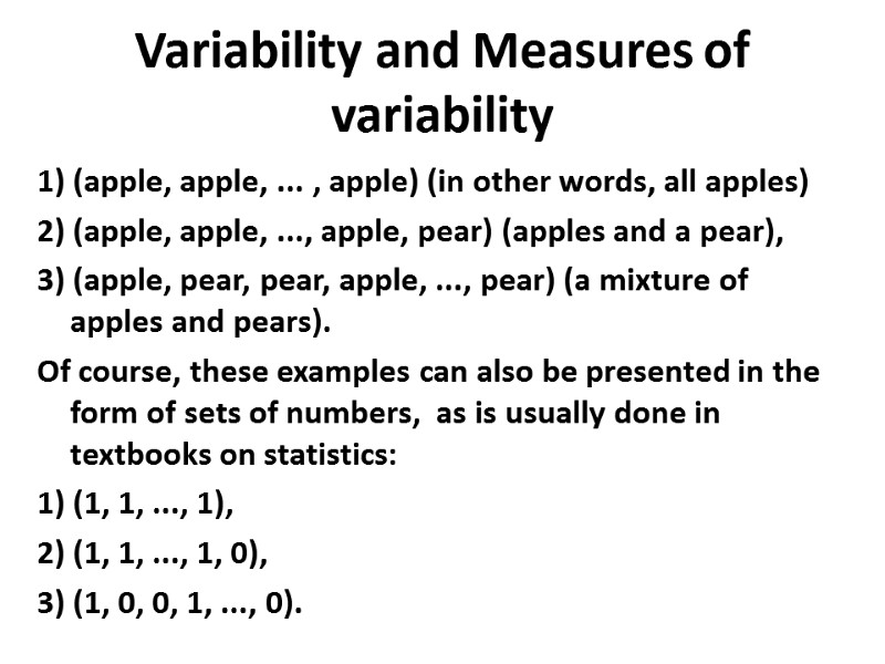
Variability and Measures of variability 1) (apple, apple, ... , apple) (in other words, all apples) 2) (apple, apple, ..., apple, pear) (apples and a pear), 3) (apple, pear, pear, apple, ..., pear) (a mixture of apples and pears). Of course, these examples can also be presented in the form of sets of numbers, as is usually done in textbooks on statistics: 1) (1, 1, ..., 1), 2) (1, 1, ..., 1, 0), 3) (1, 0, 0, 1, ..., 0).

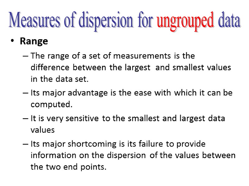
Range The range of a set of measurements is the difference between the largest and smallest values in the data set. Its major advantage is the ease with which it can be computed. It is very sensitive to the smallest and largest data values Its major shortcoming is its failure to provide information on the dispersion of the values between the two end points. Measures of dispersion for ungrouped data

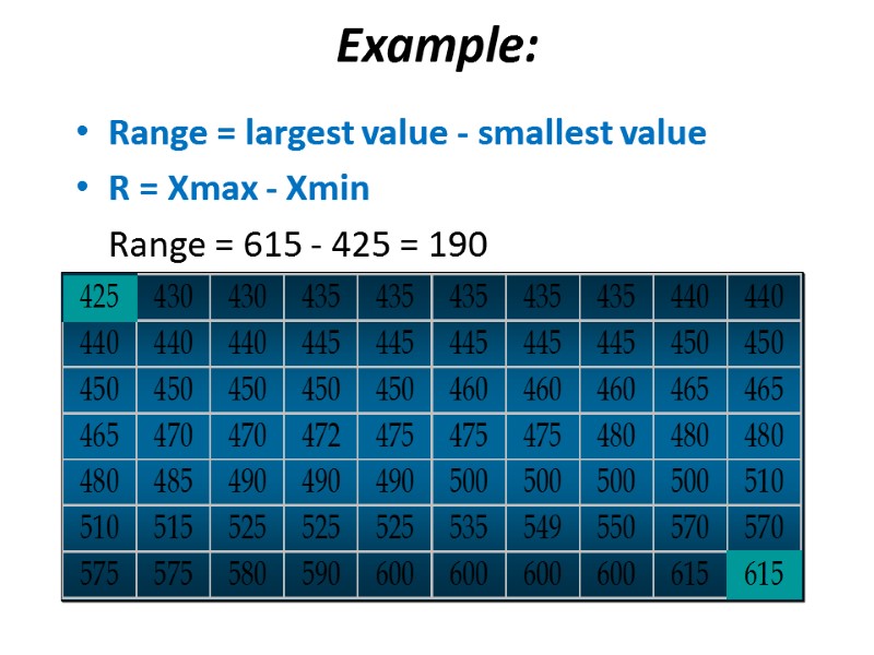
Example: Range = largest value - smallest value R = Xmax - Xmin Range = 615 - 425 = 190

Percentiles A percentile provides information about how the data are spread over the interval from the smallest value to the largest value. Admission test scores for colleges and universities are frequently reported in terms of percentiles.

The pth percentile of a data set is a value such that at least p percent of the items take on this value or less and at least (100 - p) percent of the items take on this value or more. Arrange the data in ascending order. Compute index i, the position of the pth percentile. i = (p/100)n If i is not an integer, round up. The p th percentile is the value in the i th position. If i is an integer, the p th percentile is the average of the values in positions i and i +1. Percentiles

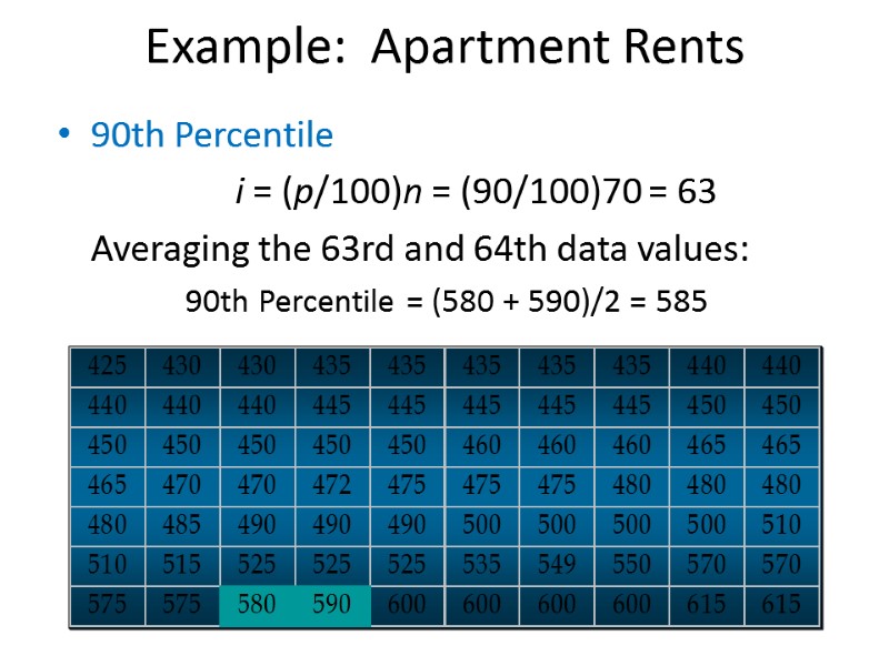
Example: Apartment Rents 90th Percentile i = (p/100)n = (90/100)70 = 63 Averaging the 63rd and 64th data values: 90th Percentile = (580 + 590)/2 = 585

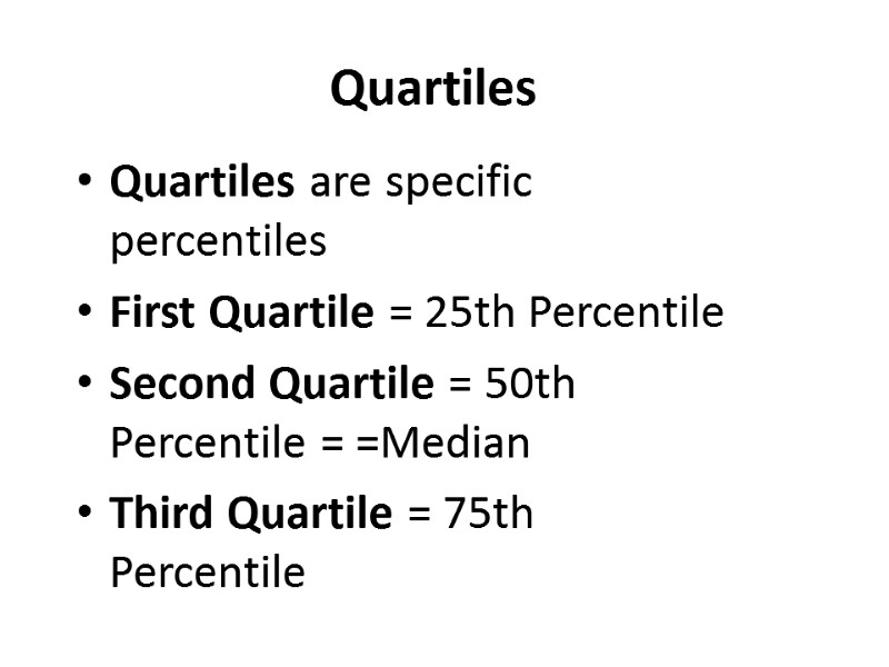
Quartiles Quartiles are specific percentiles First Quartile = 25th Percentile Second Quartile = 50th Percentile = =Median Third Quartile = 75th Percentile

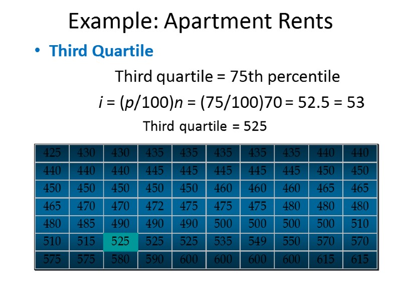
Example: Apartment Rents Third Quartile Third quartile = 75th percentile i = (p/100)n = (75/100)70 = 52.5 = 53 Third quartile = 525

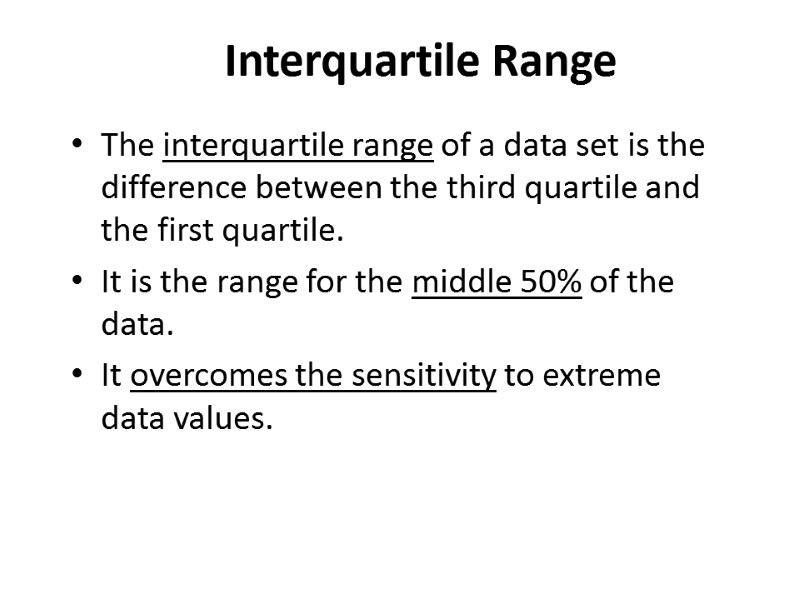
Interquartile Range The interquartile range of a data set is the difference between the third quartile and the first quartile. It is the range for the middle 50% of the data. It overcomes the sensitivity to extreme data values.

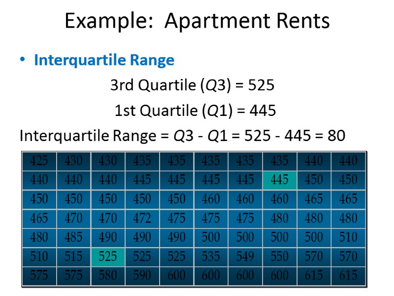
Example: Apartment Rents Interquartile Range 3rd Quartile (Q3) = 525 1st Quartile (Q1) = 445 Interquartile Range = Q3 - Q1 = 525 - 445 = 80

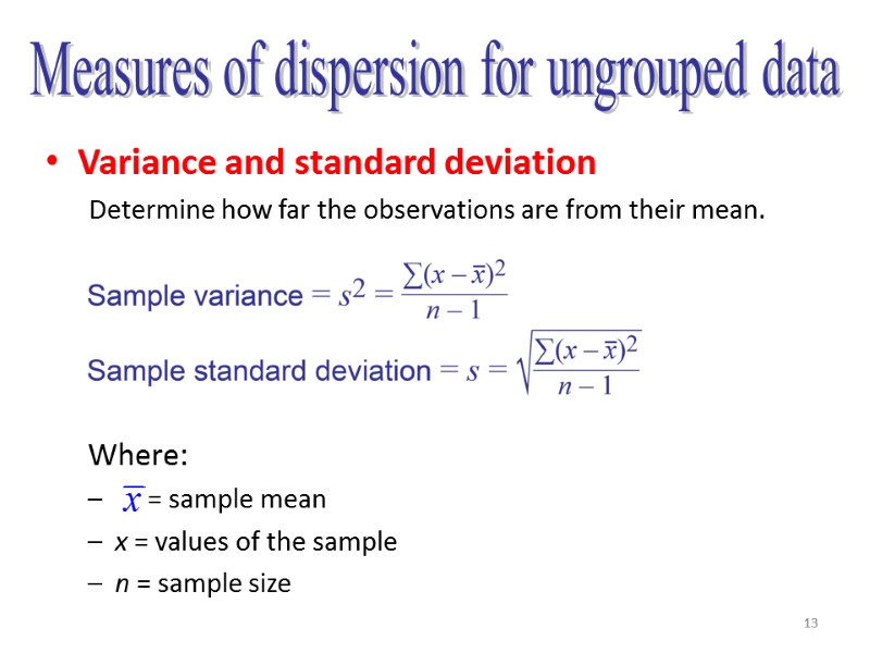
13 Variance and standard deviation Determine how far the observations are from their mean. Measures of dispersion for ungrouped data Where: = sample mean x = values of the sample n = sample size

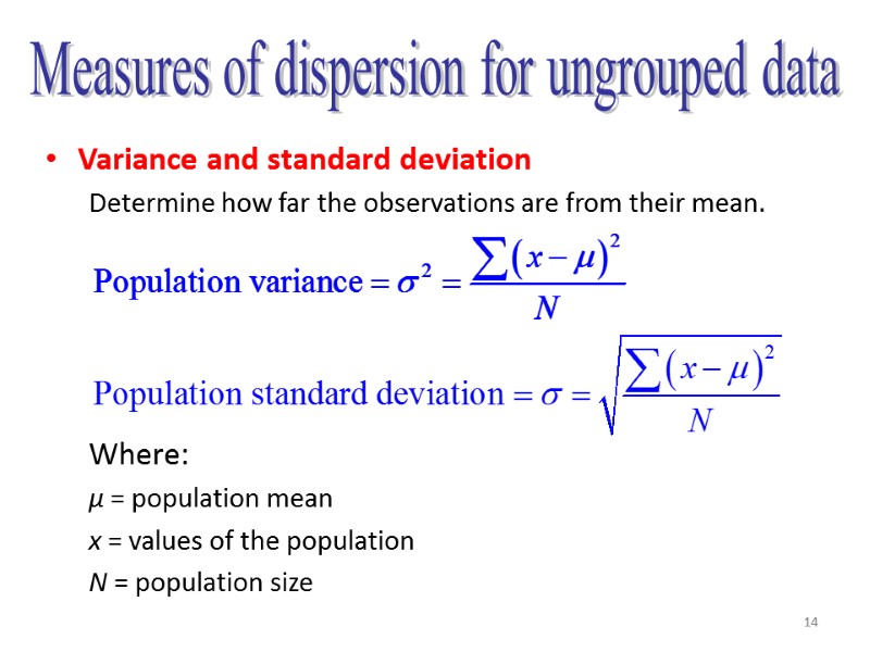
14 Variance and standard deviation Determine how far the observations are from their mean. Measures of dispersion for ungrouped data Where: μ = population mean x = values of the population N = population size

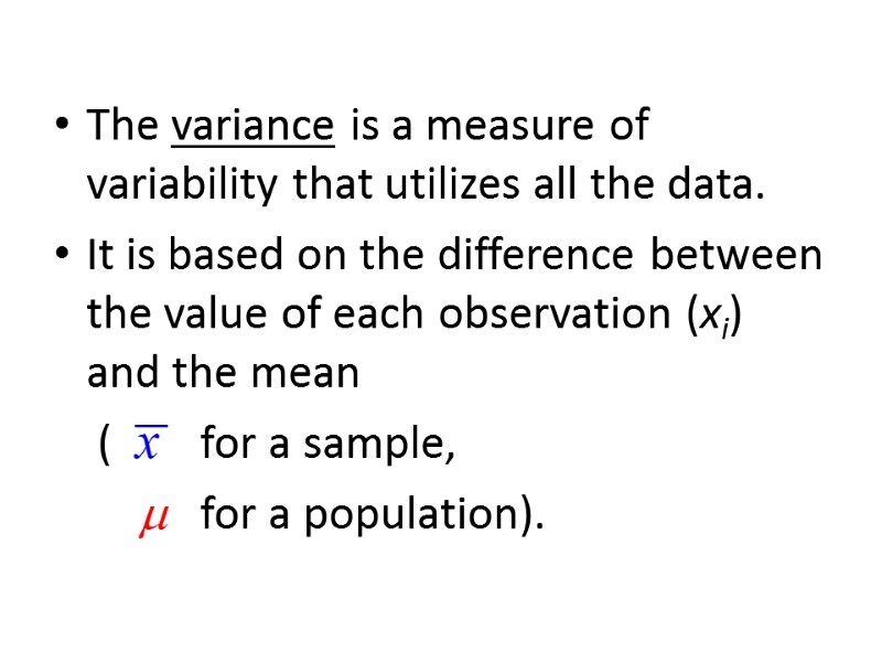
The variance is a measure of variability that utilizes all the data. It is based on the difference between the value of each observation (xi) and the mean ( for a sample, m for a population).

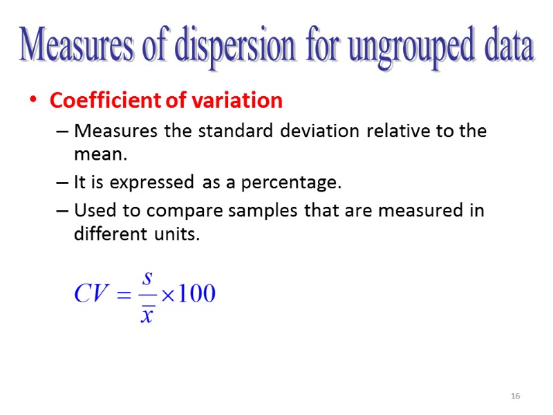
16 Coefficient of variation Measures the standard deviation relative to the mean. It is expressed as a percentage. Used to compare samples that are measured in different units. Measures of dispersion for ungrouped data

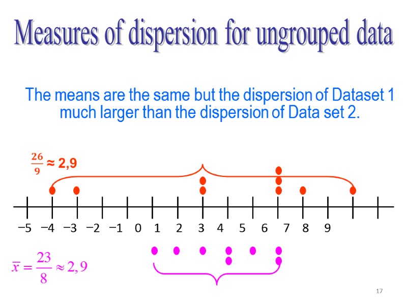
17 Measures of dispersion for ungrouped data Example - Given the following data sets: 1st: -4 -3 2 2 5 5 5 6 8 2nd : 0 1 2 3 3 4 5 5 The means are the same but the dispersion of Dataset 1 much larger than the dispersion of Data set 2.

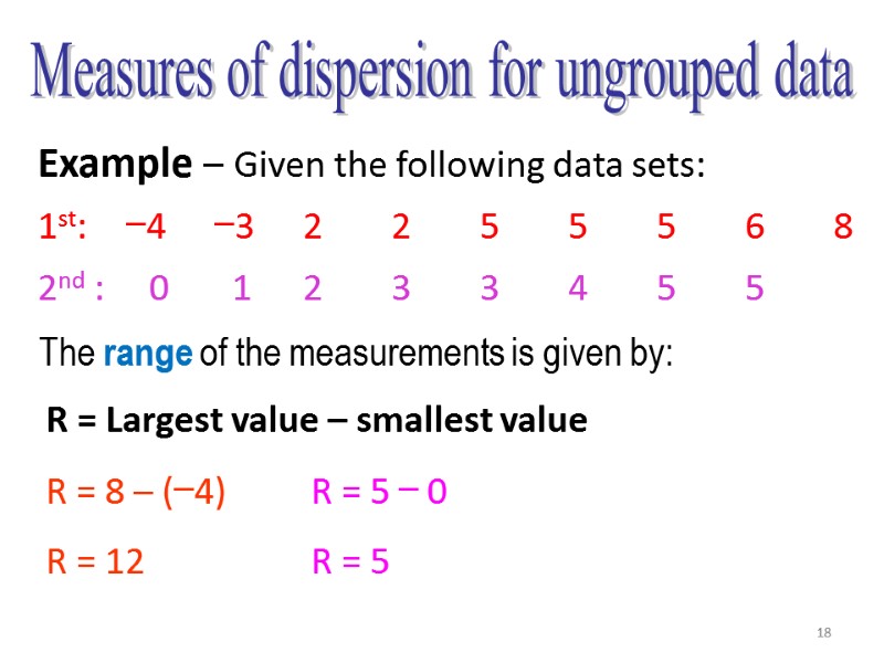
18 Measures of dispersion for ungrouped data Example – Given the following data sets: 1st: −4 −3 2 2 5 5 5 6 8 2nd : 0 1 2 3 3 4 5 5 The range of the measurements is given by: R = Largest value – smallest value R = 8 – (−4) R = 5 − 0 R = 12 R = 5

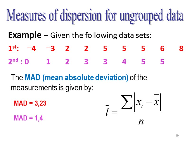
19 Measures of dispersion for ungrouped data Example – Given the following data sets: 1st: −4 −3 2 2 5 5 5 6 8 2nd : 0 1 2 3 3 4 5 5 The MAD (mean absolute deviation) of the measurements is given by: MAD = 3,23 MAD = 1,4

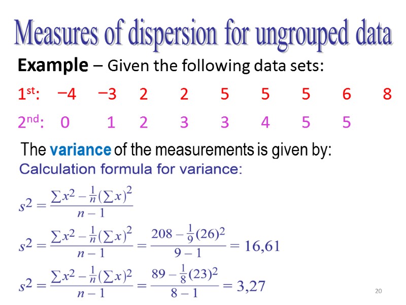
20 Measures of dispersion for ungrouped data The variance of the measurements is given by: Example – Given the following data sets: 1st: −4 −3 2 2 5 5 5 6 8 2nd: 0 1 2 3 3 4 5 5

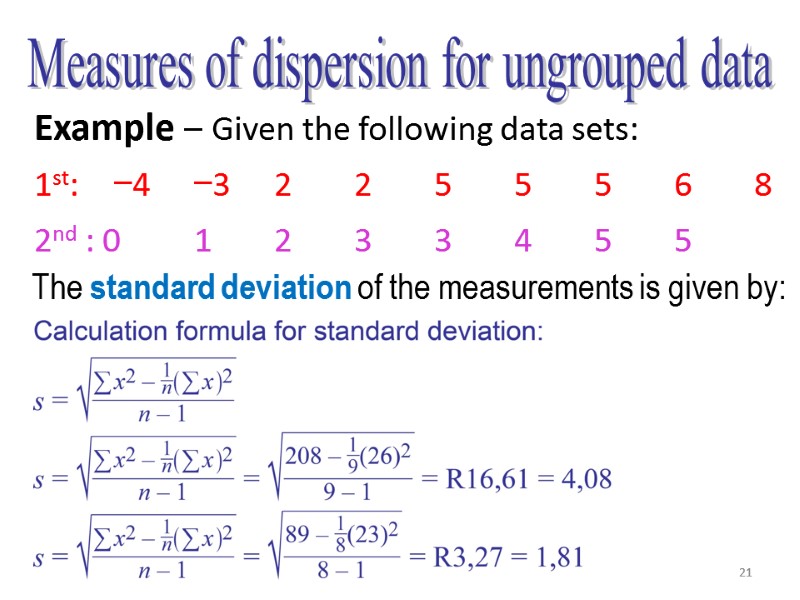
21 Measures of dispersion for ungrouped data The standard deviation of the measurements is given by: Example – Given the following data sets: 1st: −4 −3 2 2 5 5 5 6 8 2nd : 0 1 2 3 3 4 5 5

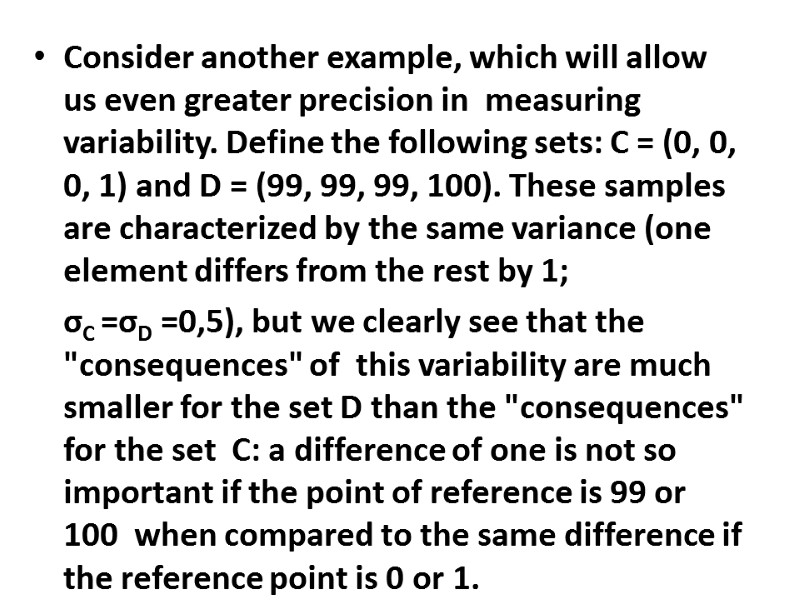
Consider another example, which will allow us even greater precision in measuring variability. Define the following sets: C = (0, 0, 0, 1) and D = (99, 99, 99, 100). These samples are characterized by the same variance (one element differs from the rest by 1; σC =σD =0,5), but we clearly see that the "consequences" of this variability are much smaller for the set D than the "consequences" for the set C: a difference of one is not so important if the point of reference is 99 or 100 when compared to the same difference if the reference point is 0 or 1.

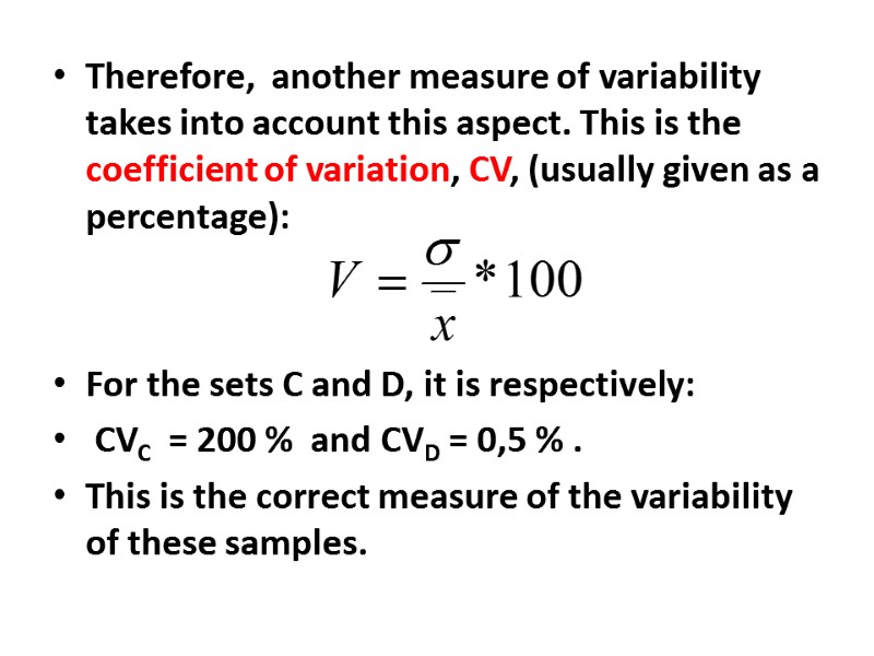
Therefore, another measure of variability takes into account this aspect. This is the coefficient of variation, СV, (usually given as a percentage): For the sets C and D, it is respectively: СVC = 200 % and СVD = 0,5 % . This is the correct measure of the variability of these samples.

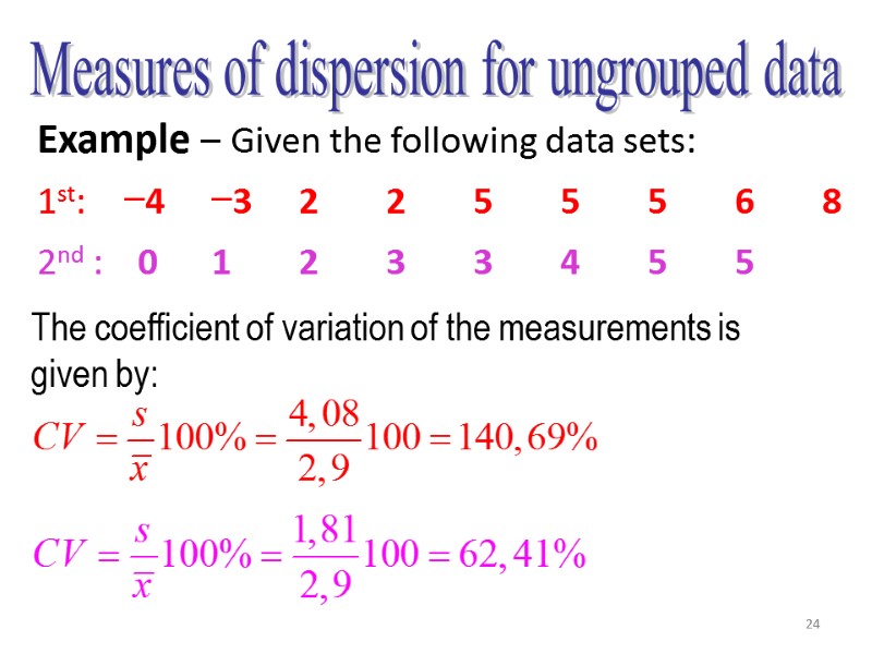
24 Measures of dispersion for ungrouped data The coefficient of variation of the measurements is given by: Example – Given the following data sets: 1st: −4 −3 2 2 5 5 5 6 8 2nd : 0 1 2 3 3 4 5 5

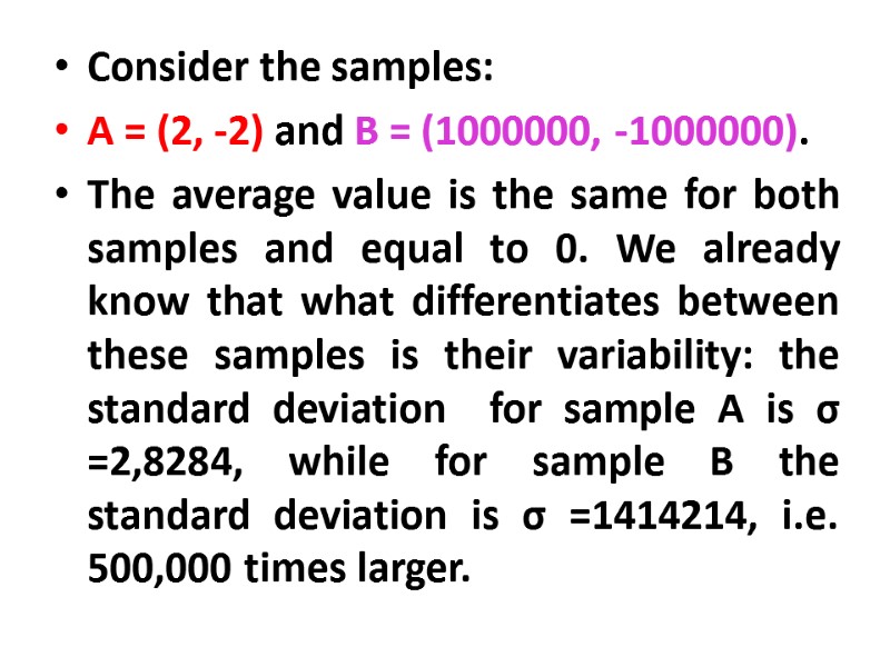
Consider the samples: A = (2, -2) and B = (1000000, -1000000). The average value is the same for both samples and equal to 0. We already know that what differentiates between these samples is their variability: the standard deviation for sample A is σ =2,8284, while for sample B the standard deviation is σ =1414214, i.e. 500,000 times larger.

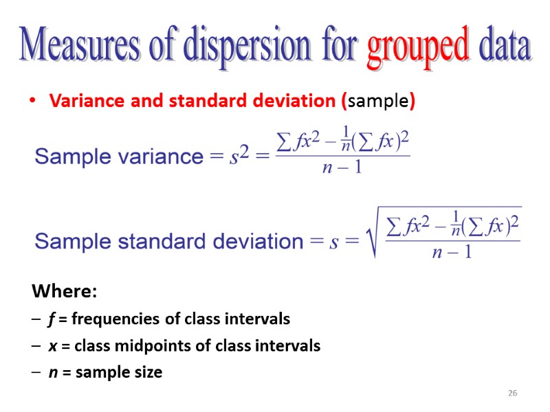
26 Variance and standard deviation (sample) Measures of dispersion for grouped data Where: f = frequencies of class intervals x = class midpoints of class intervals n = sample size

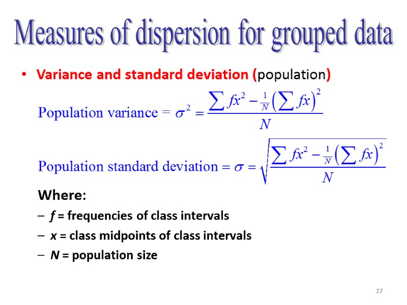
27 Variance and standard deviation (population) Measures of dispersion for grouped data Where: f = frequencies of class intervals x = class midpoints of class intervals N = population size

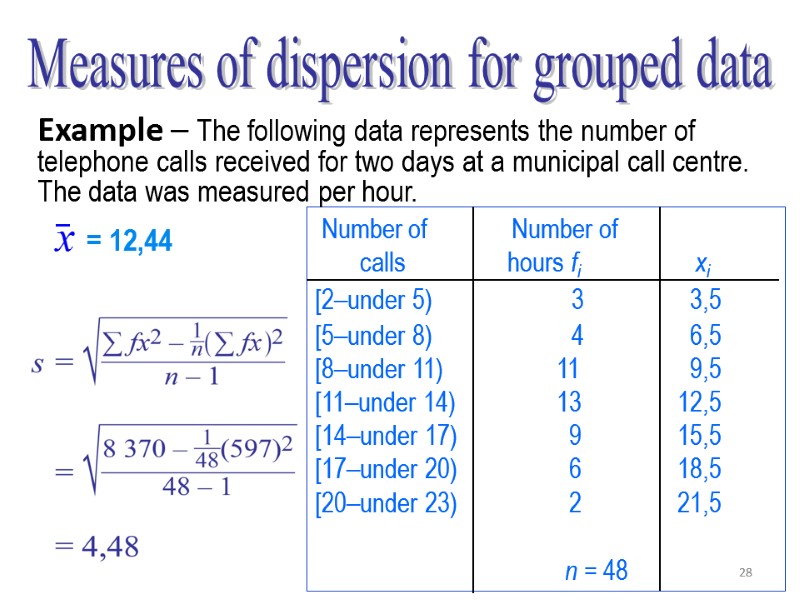
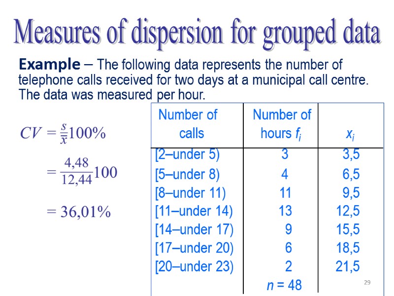
28 Number of Number of calls hours fi xi [2–under 5) 3 3,5 [5–under 8) 4 6,5 [8–under 11) 11 9,5 [11–under 14) 13 12,5 [14–under 17) 9 15,5 [17–under 20) 6 18,5 [20–under 23) 2 21,5 n = 48 Measures of dispersion for grouped data Example – The following data represents the number of telephone calls received for two days at a municipal call centre. The data was measured per hour. = 12,44

29 Number of Number of calls hours fi xi [2–under 5) 3 3,5 [5–under 8) 4 6,5 [8–under 11) 11 9,5 [11–under 14) 13 12,5 [14–under 17) 9 15,5 [17–under 20) 6 18,5 [20–under 23) 2 21,5 n = 48 Measures of dispersion for grouped data Example – The following data represents the number of telephone calls received for two days at a municipal call centre. The data was measured per hour.

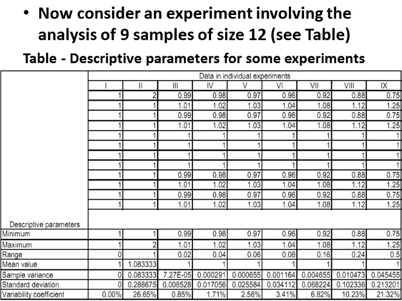
Now consider an experiment involving the analysis of 9 samples of size 12 (see Table) Table - Descriptive parameters for some experiments

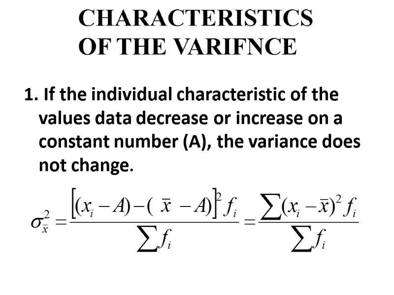
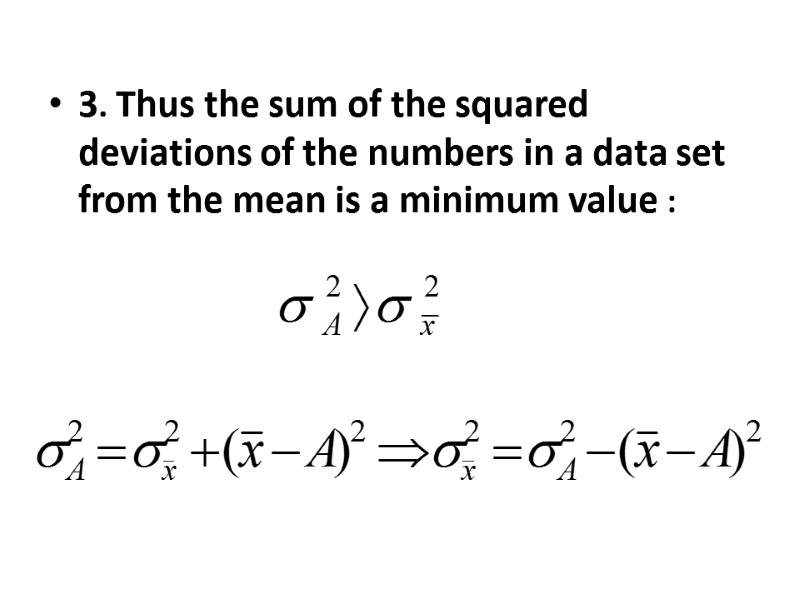
1. If the individual characteristic of the values data decrease or increase on a constant number (A), the variance does not change. CHARACTERISTICS OF THE VARIFNCE

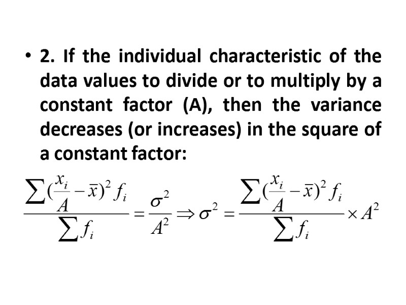
2. If the individual characteristic of the data values to divide or to multiply by a constant factor (A), then the variance decreases (or increases) in the square of a constant factor:

3. Thus the sum of the squared deviations of the numbers in a data set from the mean is a minimum value :

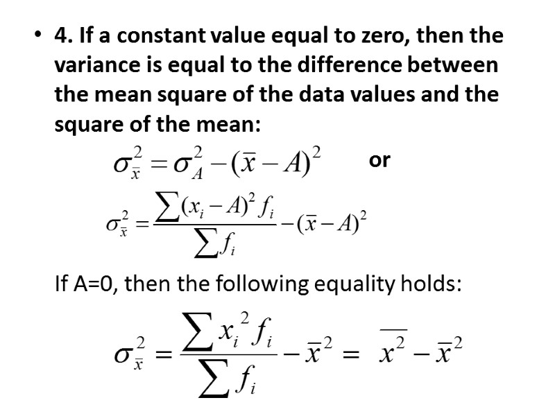
4. If a constant value equal to zero, then the variance is equal to the difference between the mean square of the data values and the square of the mean: or If A=0, then the following equality holds:

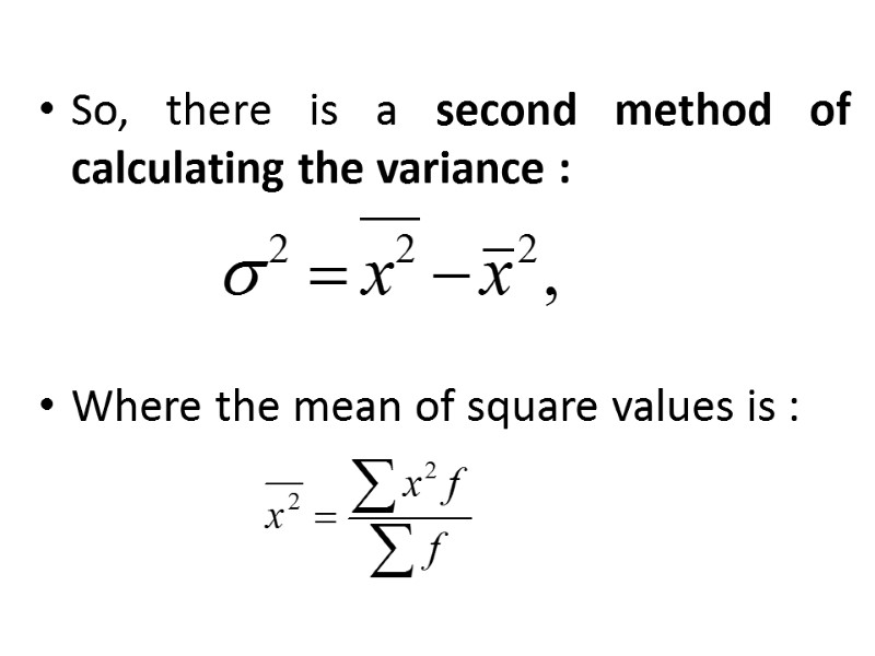
So, there is a second method of calculating the variance : Where the mean of square values is :

The short-cut formula has been derived for calculating the sample variance. This is handy when the data being evaluated number more than a few items. This equation is the short-cut formula used to compute the sample variance. The sample standard deviation is computed by taking the square root of this variance.

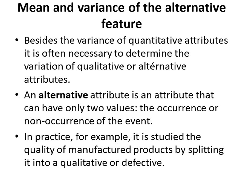
Mean and variance of the alternative feature Besides the variance of quantitative attributes it is often necessary to determine the variation of qualitative or altérnative attributes. An alternative attribute is an attribute that can have only two values: the occurrence or non-occurrence of the event. In practice, for example, it is studied the quality of manufactured products by splitting it into a qualitative or defective.

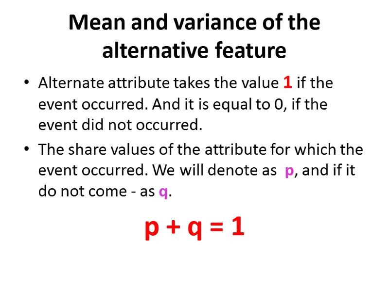
Mean and variance of the alternative feature Alternate attribute takes the value 1 if the event occurred. And it is equal to 0, if the event did not occurred. The share values ​​of the attribute for which the event occurred. We will denote as p, and if it do not come - as q. p + q = 1

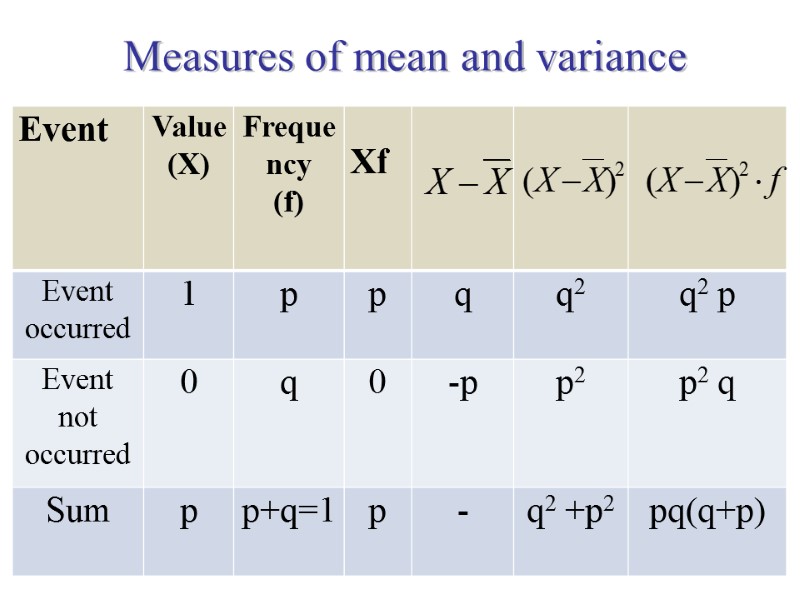
Measures of mean and variance

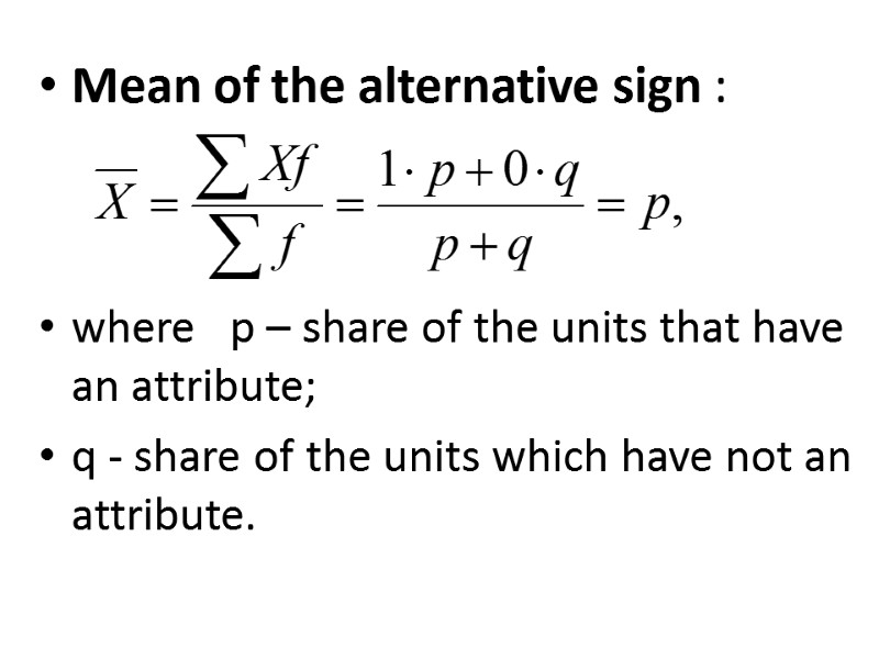
Mean of the alternative sign : where р – share of the units that have an attribute; q - share of the units which have not an attribute.

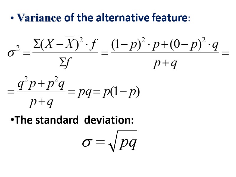
Variance of the alternative feature: The standard deviation:

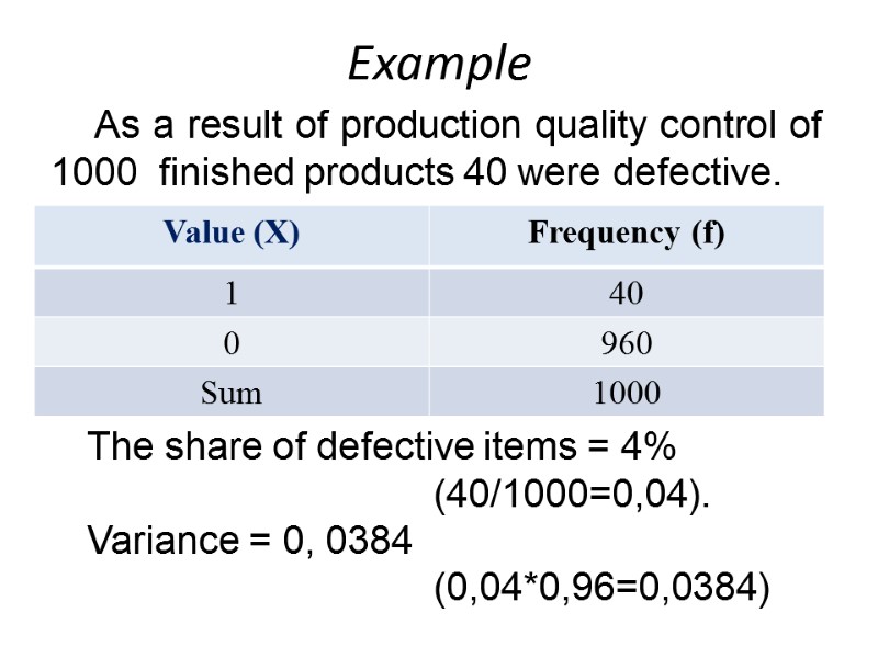
Example As a result of production quality control of 1000 finished products 40 were defective. The share of defective items = 4% (40/1000=0,04). Variance = 0, 0384 (0,04*0,96=0,0384)

Further Measures of variations you have calculated independently

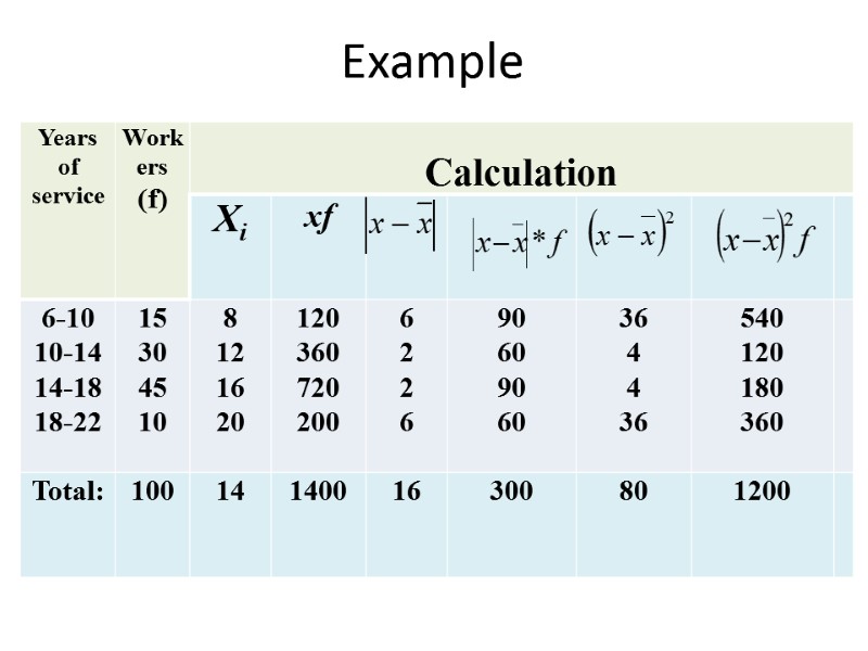
Example

Example

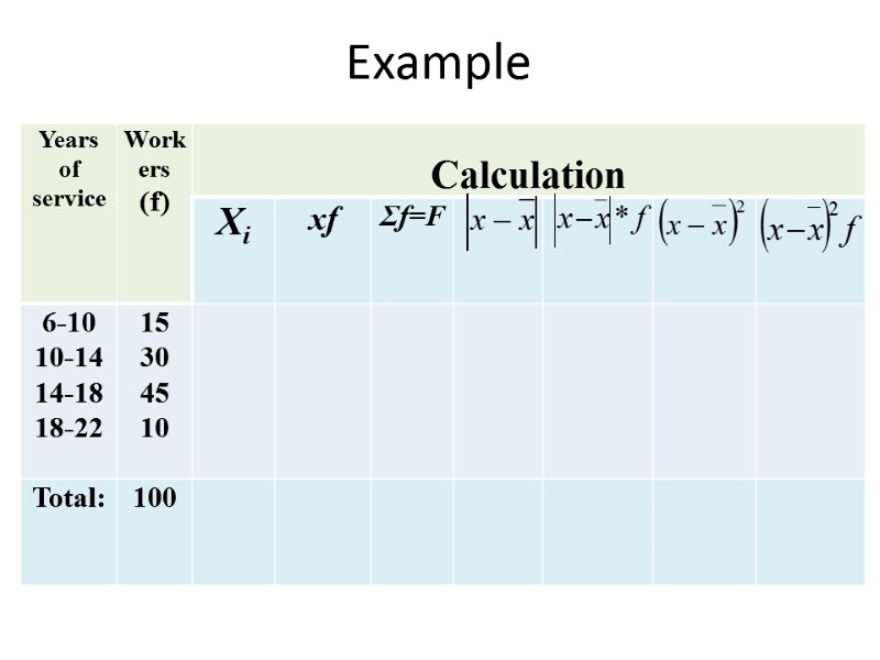
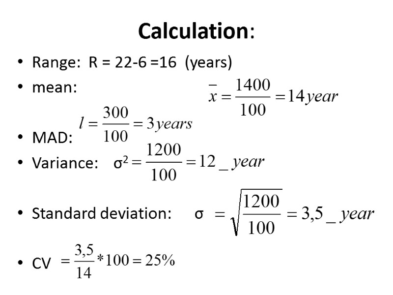
Calculation: Range: R = 22-6 =16 (years) mean: MAD: Variance: σ2 Standard deviation: σ CV