1 Fundamental Principles 2 of Process Control Motivation

1. Fundamental Principles 2. of Process Control Motivation for Automatic Process Control • Safety First: – people, environment, equipment • The Profit Motive: – meeting final product specs – minimizing waste production – minimizing environmental impact – minimizing energy use – maximizing overall production rate

“Loose” Control Costs Money • It takes more material to make a product thicker, so greatest profit is to operate as close to the minimum thickness constraint as possible without going under • It takes more processing to remove impurities, so greatest profit is to operate as close to the maximum impurities constraint as you can without going over

Tight Control = Most Profitable Operation • A well controlled process has less variability in the measured process variable, so the process can be operated close to the profitable constraint

Consider heating a house Terminology Control Objective Measured Process Variable Set point Controller Output Manipulated Variable Disturbances

Automatic Control is Measurement Computation Action • Is house cooler than set point? ( TSetpoint Thouse > 0 ) Action open fuel valve • Is house warmer than set point? ( TSetpoint THouse < 0 ) Action close fuel valve

Components of a Control Loop Home heating control block diagram

General Control Loop Block Diagram

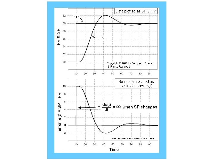
Starting at the far right of the control loop block diagram: • a sensor measures and transmits the current value of the process variable, PV, back to the controller (the 'controller wire in') • controller error at current time t is computed as set point minus measured process variable, or e(t) = SP – PV • the controller uses this e(t) in a control algorithm to compute a new controller output signal, CO • the CO signal is sent to the final control element (e. g. valve, pump, heater, fan) causing it to change (the 'controller wire out') • the change in the final control element (FCE) causes a change in a manipulated variable • the change in the manipulated variable (e. g. flow rate of liquid or gas) causes a change in the PV The goal of the controller is to make e(t) = 0 (or PV = SP) in spite of unplanned and unmeasured disturbances. •

On/Off Control – The Simplest Controller • For on/off control, the final control element is either completely open/on/maximum or closed/off/minimum • To protect the final control element from wear, a dead band or upper and a lower set point is used • As long as the measured variable remains between these limits, no changes in control action are made

Usefulness of On/Off Control • On/off with dead band is useful for home appliances such as furnaces, air conditioners, ovens and refrigerators • For most industrial applications, on/off is too limiting (think about riding in a car that has on/off cruise control)

Intermediate Value Control and PID • Industry requires controllers that permit tighter control with less oscillation in the measured process variable • These algorithms: – compute a complete range of actions between full on/off – require a final control element that can assume intermediate positions between full on/off • Example final control elements include process valves, variable speed pumps and compressors, and electronic heating elements

Intermediate Value Control and PID • Popular intermediate value controller is PID (proportional-integral-derivative) controller • PID computes a controller output signal based on control error: Proportional Integral Derivative term where: y(t) = measured process variable u(t) = controller output signal ubias = controller bias or null value e(t) = controller error = ysetpoint – y(t) KC = controller gain (a tuning parameter) I = controller reset time (a tuning parameter) D = controller derivative time (a tuning parameter)

5. P-Only => The Simplest PID Controller The Proportional Controller • The simplest PID controller is proportional or P-Only control • It can compute intermediate control values between 0 – 100%

The Gravity Drained Tanks Control Loop • Measurement, computation and control action repeat every loop sample time: – a sensor measures the liquid level in the lower tank – this measurement is subtracted from the set point level to determine a control error e(t) = ysetpoint – y(t) – the controller computes an output based on this error and it is transmitted to the valve, causing it to move – this causes the liquid flow rate into the top tank to change, which ultimately changes the level in the lower tank • The goal is to eliminate the controller error by making the measured level in the lower tank equal the set point level

P-Only Control • The controller computes an output signal every sample time: u(t) = ubias + KC e(t) where u(t) ubias e(t) KC = controller output = the controller bias = controller error = set point – measurement = ysetpoint – y(t) = controller gain (a tuning parameter) • controller gain, KC steady state process gain, KP • a larger KC means a more active controller • like KP , controller gain has a size, sign and units

Controller Gain, KC, From Correlations • P-Only control has one adjustable or tuning parameter, KC u(t) = ubias + KC e(t) • KC sets the activity of the controller to changes in error, e(t) – if KC is small, the controller is sluggish – If KC is large, the controller is aggressive

Understanding Controller Bias, ubias • Thought Experiment: – Consider P-Only cruise control where u(t) is the flow of gas – Suppose velocity set point = measured velocity = 70 km/h – Since y(t) = ysetpoint then e(t) = 0 and P-Only controller is u(t) = ubias + 0 – If ubias were set to zero, then the flow of gas to the engine would be zero even though the car is going 70 km/h • If the car is going 70 km/h, there clearly is a baseline flow of gas • This baseline controller output is the bias or null value

Understanding Controller Bias, ubias • In the thought experiment, the bias is the flow of gas which, in open loop, causes the car to travel the design velocity of 70 km/h when the disturbances are at their normal or expected values • In general, ubias is the value of the controller output that, in open loop, causes the measured process variable to maintain steady state at the design level of operation when the process disturbances are at their design or expected values • Controller bias is not normally adjusted once the controller is put in automatic

Reverse Action, Direct Action and Control Action • If KP is positive and the process variable is too high, the controller decreases the controller output to correct the error => The controller action is the reverse of the problem When KP is positive, the controller is reverse acting When KP is negative, the controller is direct acting • Since KC always has the same sign as KP , then KP and KC positive reverse acting KP and KC negative direct acting

Reverse Acting, Direct Acting and Control Action • Most commercial controllers require you to enter • a positive KC • The sign (or action) of the controller is specified by entering the controller as reverse or direct acting • If the wrong control action is entered, the controller will drive the valve to full open or closed until the entry is corrected

Offset - The Big Disadvantage of P-Only Control • Big advantage of P-Only control: => only one tuning parameter so it’s easy to find “best” tuning • Big disadvantage: => the controller permits offset

Offset - The Big Disadvantage of P-Only Control • Offset occurs under P-Only control when the set point and/or disturbances are at values other than that used as the design level of operation (that used to determine ubias) u(t) = ubias + KC e(t) • How can the P-Only controller compute a value for u(t) that is different from ubias at steady state? • The only way is if e(t) 0

Offset and KC As KC increases: Offset decreases Oscillatory behavior increases

Pulse Test • Pulse test is two step tests performed in rapid succession • Desirable: starts from and returns to an initial steady state • Undesirable: data generated on one side of this steady state (which presumably is design level of operation)

P - control Control-equation Electrical circuit Step-response

I - control Control-equation Electrical circuit Step-response

PI - control Control-equation Electrical circuit Step-response

PD - control Control-equation Electrical circuit Step-response

PID - control Control-equation Electrical circuit Step-response

Step response Comparison between different types of control Time

Block-Diagramm PID - Control Input Control Bias Ue Set Value Us

Circuit -Diagramm PID - Control P-Element Inverting amplifier I-Element Summing amplifier D-Element