01cd0dd08b533bc63ee04769d3282d36.ppt
- Количество слайдов: 46
1 CHAPTER 7 Subjective Probability and Bayesian Inference
7. 1. Subjective Probability w Personal evaluation of probability by individual decision maker w Uncertainty exists for decision maker: probability is just a way of measuring it w In dealing with uncertainty, a coherent decision maker effectively uses subjective probability 2
7. 2. Assessment of Subjective Probabilities Simplest procedure: Specify the set of all possible events, w ask the decision maker to directly estimate probability of each event w Not a good approach from psychological point of view w Not easy to conceptualize, especially for DM not familiar with probability w 3
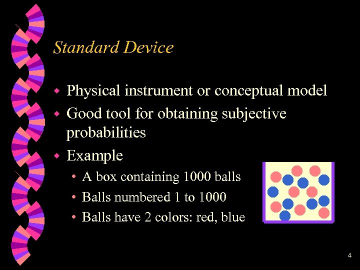
Standard Device Physical instrument or conceptual model w Good tool for obtaining subjective probabilities w Example w • A box containing 1000 balls • Balls numbered 1 to 1000 • Balls have 2 colors: red, blue 4
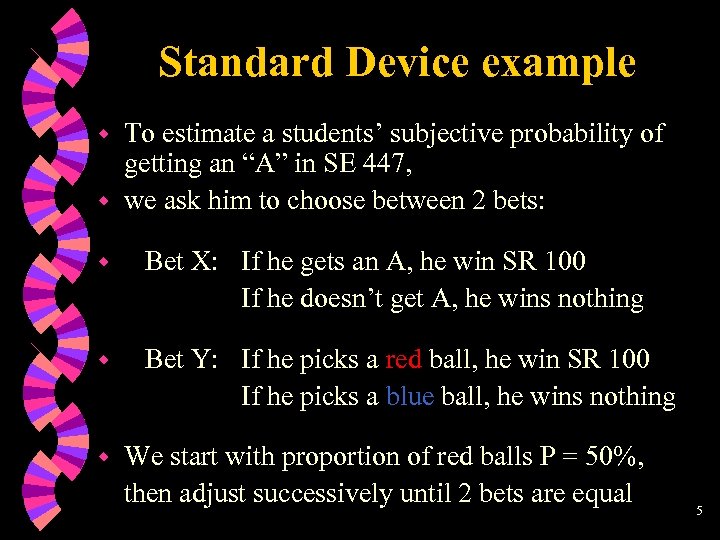
Standard Device example To estimate a students’ subjective probability of getting an “A” in SE 447, w we ask him to choose between 2 bets: w w Bet X: If he gets an A, he win SR 100 If he doesn’t get A, he wins nothing w Bet Y: If he picks a red ball, he win SR 100 If he picks a blue ball, he wins nothing w We start with proportion of red balls P = 50%, then adjust successively until 2 bets are equal 5
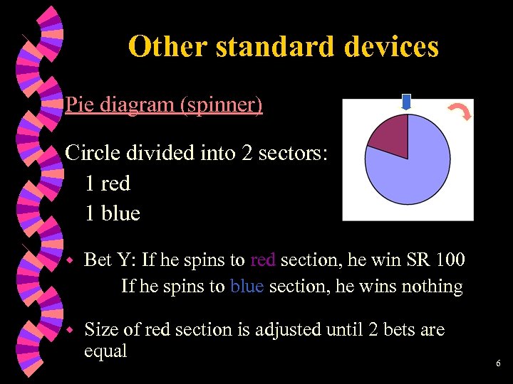
Other standard devices Pie diagram (spinner) Circle divided into 2 sectors: 1 red 1 blue w Bet Y: If he spins to red section, he win SR 100 If he spins to blue section, he wins nothing w Size of red section is adjusted until 2 bets are equal 6
Subjective Probability Bias w Standard device must be easy to perceive, to avoid introducing bias 2 kinds of bias: Task bias: resulting from assessment method (standard device) w Conceptual bias: resulting from mental procedures (heuristics) used by individuals to process information w 7
Mental Heuristics Causing Bias 1. Representativeness • • • 2. Availability • 3. Limits of memory and imagination Adjustment & anchoring • • w If x highly represents set A, high probability is given that X A Frequency (proportion) ignored Sample size ignored Starting from obvious reference point, then adjusting for new values. Anchoring: adjustment is typically not enough Overconfidence • Underestimating variance 8
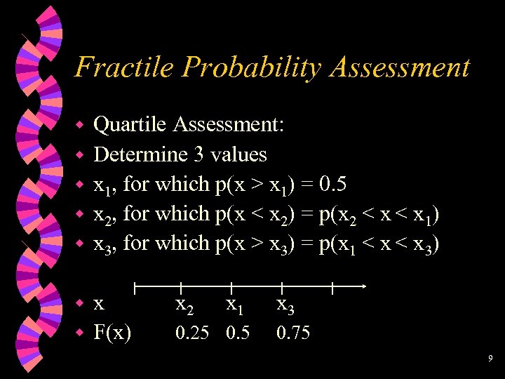
Fractile Probability Assessment w w w Quartile Assessment: Determine 3 values x 1, for which p(x > x 1) = 0. 5 x 2, for which p(x < x 2) = p(x 2 < x 1) x 3, for which p(x > x 3) = p(x 1 < x 3) x w F(x) w x 2 x 1 0. 25 0. 5 x 3 0. 75 9
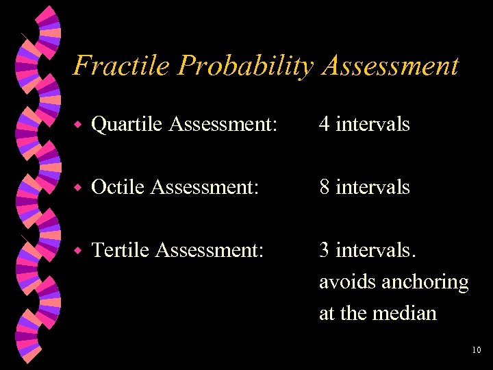
Fractile Probability Assessment w Quartile Assessment: 4 intervals w Octile Assessment: 8 intervals w Tertile Assessment: 3 intervals. avoids anchoring at the median 10
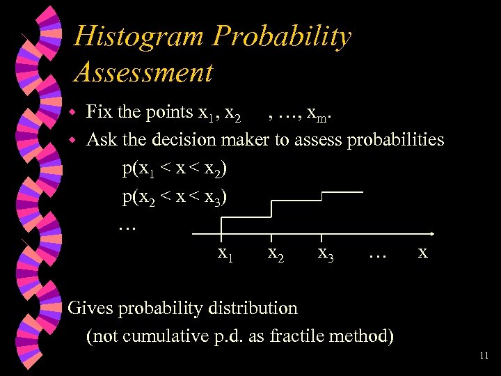
Histogram Probability Assessment Fix the points x 1, x 2 , …, xm. w Ask the decision maker to assess probabilities p(x 1 < x 2) p(x 2 < x 3) … x 1 x 2 x 3 … x w Gives probability distribution (not cumulative p. d. as fractile method) 11
Assessment Methods & Bias No evidence to favor either fractile or histogram methods w One factor that reinforces anchoring bias is self-consistency w Bias can be reduced by “pre-assessment conditioning”: training, for/against arguments w The act of probability assessment causes a re-evaluation of uncertainty w 12
7. 3. Impact of New Information (Bayes’ Theorem) w After developing subjective probability distribution w Assume new information becomes available Example: new data is collected w According to coherence principle, DM must take new information in consideration, thus Subjective probability must be revised w How? using Bayes’ theorem 13
Bayes’ Theorem Example w Suppose your subjective probability distribution for weather tomorrow is: • chances of being sunny • chances of being not sunny P(S) = 0. 6 P(N) = 0. 4 w If the TV weather forecast predicted a cloudy day tomorrow. How should you change P(S)? w Assume we are dealing with mutually exclusive and collectively exhaustive events such as sunny or not sunny. 14
Impact of Information w We assume the weather forecaster predicts either • cloudy day C, or • bright day B. w To change P(S), we use the joint probability = conditional probability * marginal probability • P(C, S) = P(C|S)P(B, S) = P(B|S)P(S) • P(C, N) = P(C|N)P(N) P(B, N)= P(B|N)P(N) 15
Impact of Information To obtain j. p. m. f we need the conditional probabilities P(C|S) and P(C|N). w These can be obtained from historical data. How? w w In past 100 sunny days, cloudy forecast in 20 days P(C|S) = 0. 2 P(B|S) = 0. 8 w In past 100 cloudy days, cloudy forecast in 90 days P(C|N) = 0. 9 P(B|N) = 0. 1 16
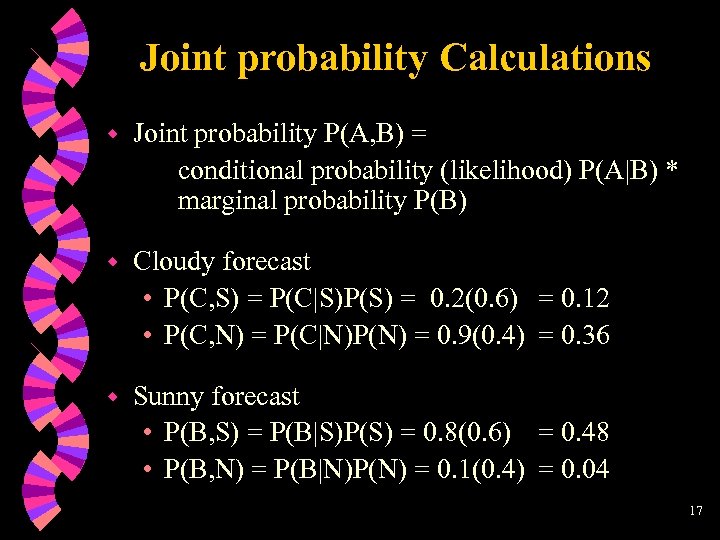
Joint probability Calculations w Joint probability P(A, B) = conditional probability (likelihood) P(A|B) * marginal probability P(B) w Cloudy forecast • P(C, S) = P(C|S)P(S) = 0. 2(0. 6) = 0. 12 • P(C, N) = P(C|N)P(N) = 0. 9(0. 4) = 0. 36 w Sunny forecast • P(B, S) = P(B|S)P(S) = 0. 8(0. 6) = 0. 48 • P(B, N) = P(B|N)P(N) = 0. 1(0. 4) = 0. 04 17
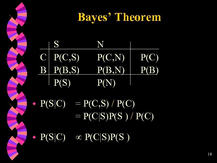
Bayes’ Theorem S C P(C, S) B P(B, S) P(S) N P(C, N) P(B, N) P(C) P(B) w P(S|C) = P(C, S) / P(C) = P(C|S)P(S ) / P(C) w P(S|C) P(C|S)P(S ) 18
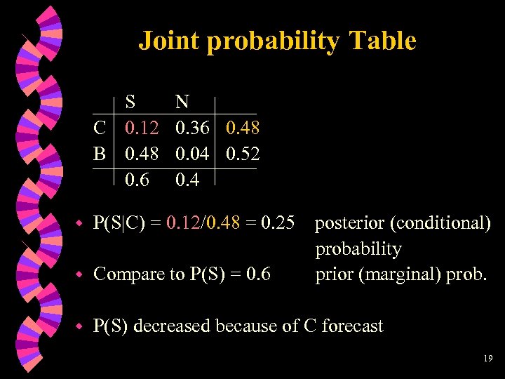
Joint probability Table S C 0. 12 B 0. 48 0. 6 N 0. 36 0. 48 0. 04 0. 52 0. 4 w P(S|C) = 0. 12/0. 48 = 0. 25 posterior (conditional) probability prior (marginal) prob. w Compare to P(S) = 0. 6 w P(S) decreased because of C forecast 19
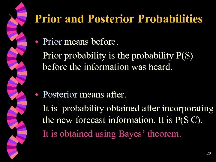
Prior and Posterior Probabilities w Prior means before. Prior probability is the probability P(S) before the information was heard. w Posterior means after. It is probability obtained after incorporating the new forecast information. It is P(S|C). It is obtained using Bayes’ theorem. 20
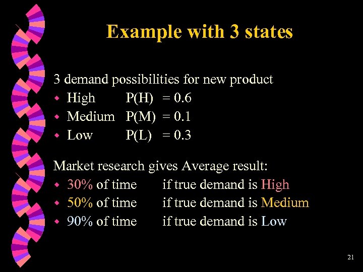
Example with 3 states 3 demand possibilities for new product w High P(H) = 0. 6 w Medium P(M) = 0. 1 w Low P(L) = 0. 3 Market research gives Average result: w 30% of time if true demand is High w 50% of time if true demand is Medium w 90% of time if true demand is Low 21
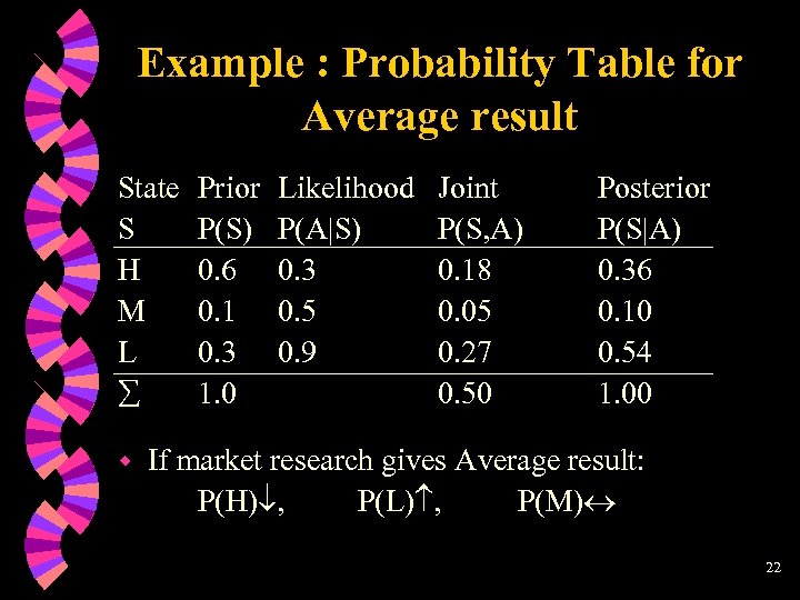
Example : Probability Table for Average result State S H M L w Prior P(S) 0. 6 0. 1 0. 3 1. 0 Likelihood P(A|S) 0. 3 0. 5 0. 9 Joint P(S, A) 0. 18 0. 05 0. 27 0. 50 Posterior P(S|A) 0. 36 0. 10 0. 54 1. 00 If market research gives Average result: P(H) , P(L) , P(M) 22
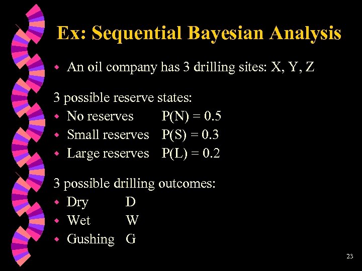
Ex: Sequential Bayesian Analysis w An oil company has 3 drilling sites: X, Y, Z 3 possible reserve states: w No reserves P(N) = 0. 5 w Small reserves P(S) = 0. 3 w Large reserves P(L) = 0. 2 3 possible drilling outcomes: w Dry D w Wet W w Gushing G 23
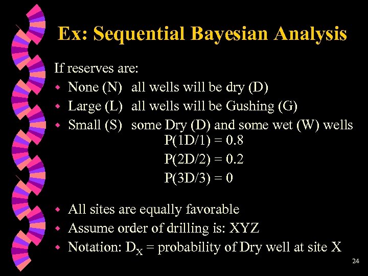
Ex: Sequential Bayesian Analysis If reserves are: w None (N) all wells will be dry (D) w Large (L) all wells will be Gushing (G) w Small (S) some Dry (D) and some wet (W) wells P(1 D/1) = 0. 8 P(2 D/2) = 0. 2 P(3 D/3) = 0 All sites are equally favorable w Assume order of drilling is: XYZ w Notation: DX = probability of Dry well at site X w 24
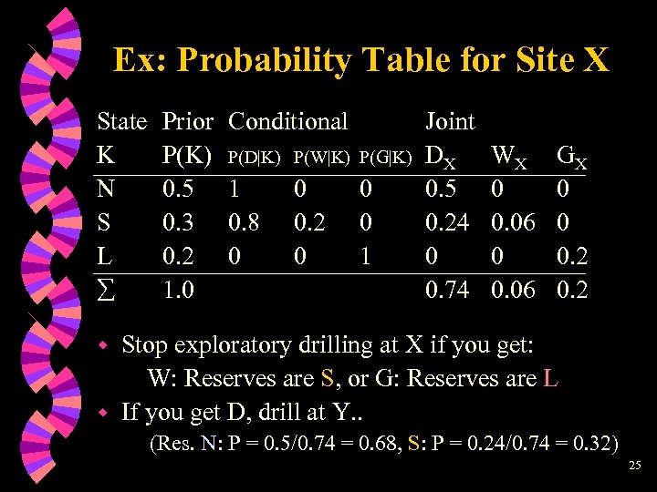
Ex: Probability Table for Site X State K N S L Prior P(K) 0. 5 0. 3 0. 2 1. 0 Conditional P(D|K) P(W|K) P(G|K) 1 0. 8 0 0 0. 2 0 0 0 1 Joint DX 0. 5 0. 24 0 0. 74 WX 0 0. 06 GX 0 0 0. 2 Stop exploratory drilling at X if you get: W: Reserves are S, or G: Reserves are L w If you get D, drill at Y. . w (Res. N: P = 0. 5/0. 74 = 0. 68, S: P = 0. 24/0. 74 = 0. 32) 25
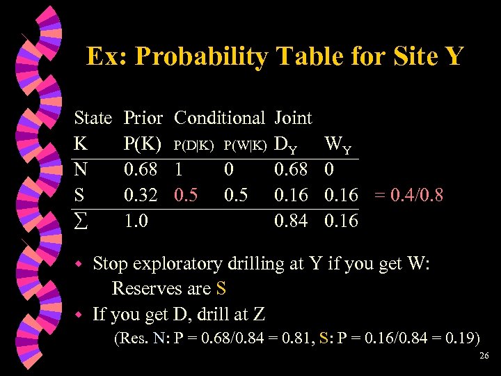
Ex: Probability Table for Site Y State K N S Prior Conditional Joint P(K) P(D|K) P(W|K) DY 0. 68 1 0 0. 68 0. 32 0. 5 0. 16 1. 0 0. 84 WY 0 0. 16 = 0. 4/0. 8 0. 16 Stop exploratory drilling at Y if you get W: Reserves are S w If you get D, drill at Z w (Res. N: P = 0. 68/0. 84 = 0. 81, S: P = 0. 16/0. 84 = 0. 19) 26
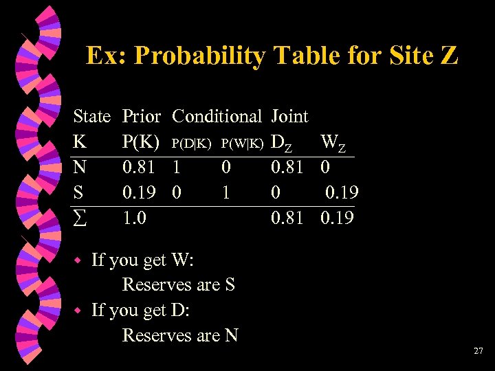
Ex: Probability Table for Site Z State K N S Prior Conditional Joint P(K) P(D|K) P(W|K) DZ 0. 81 1 0 0. 81 0. 19 0 1. 0 0. 81 If you get W: Reserves are S w If you get D: Reserves are N WZ 0 0. 19 w 27
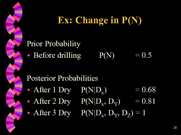
Ex: Change in P(N) Prior Probability w Before drilling P(N) = 0. 5 Posterior Probabilities w After 1 Dry P(N|Dx) = 0. 68 w After 2 Dry P(N|Dx, DY) = 0. 81 w After 3 Dry P(N|Dx, DY, DZ) = 1 28
7. 4. Conditional Independence Two events, A and B, are independent iff: w P(A, B) = P(A)*P(B) Implying w P(A|B) = P(A) w P(B|A) = P(B) Posterior probability is the same the prior w New information about 1 event does not affect the probability of the other w 29
Conditional Independence Two events, A and B, are conditionally independent iff: w P(A, B) P(A)*P(B) But their conditional probabilities on a 3 rd event, C, are independent w P(A, B|C) = P(A|C)*P(B|C) w Useful property in Bayesian analysis 30
Ex: Horse Race Probability Horse named WR will race at 3: 00 p. m. Probability of WR winning P(WR) depends on track condition Firm (F) w Soft (S) w P(F) = 0. 3 P(S) = 0. 7 P(WR|F) = 0. 9 P(WR|S) = 0. 2 31
Ex: Horse Race Probability w Given the results of 2 previous races w At 1: 30, horse named MW won the race P(MW|F) = 0. 8 P(MW|S) = 0. 4 w At 2: 00, horse named AJ won the race P(AJ|F) = 0. 9 P(AJ|S) = 0. 5 w What the new WR win probability P(WR|MW, AJ)? 32
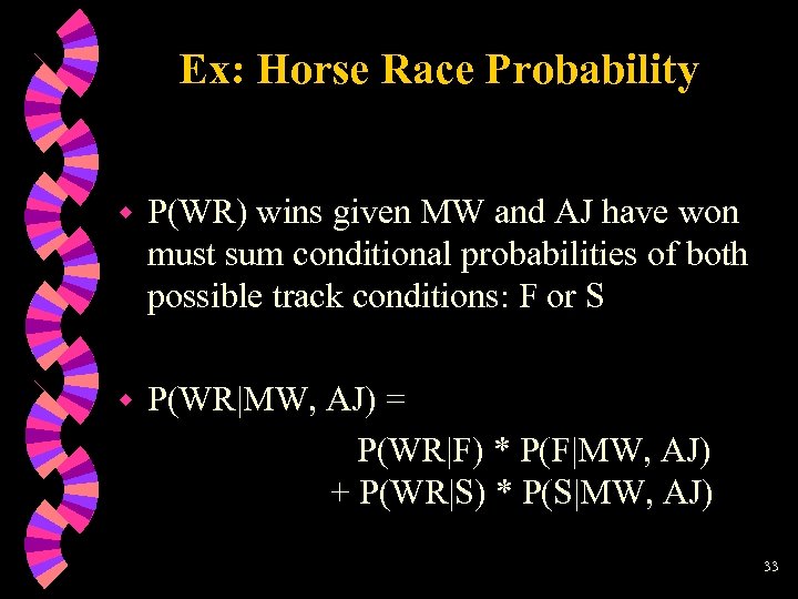
Ex: Horse Race Probability w P(WR) wins given MW and AJ have won must sum conditional probabilities of both possible track conditions: F or S w P(WR|MW, AJ) = P(WR|F) * P(F|MW, AJ) + P(WR|S) * P(S|MW, AJ) 33
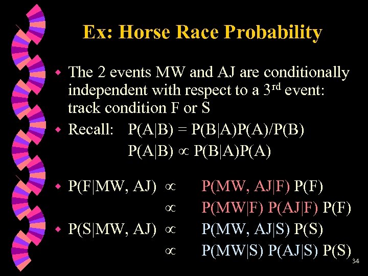
Ex: Horse Race Probability The 2 events MW and AJ are conditionally independent with respect to a 3 rd event: track condition F or S w Recall: P(A|B) = P(B|A)P(A)/P(B) P(A|B) P(B|A)P(A) w P(F|MW, AJ) w P(S|MW, AJ) w P(MW, AJ|F) P(MW|F) P(AJ|F) P(MW, AJ|S) P(MW|S) P(AJ|S) P(S) 34
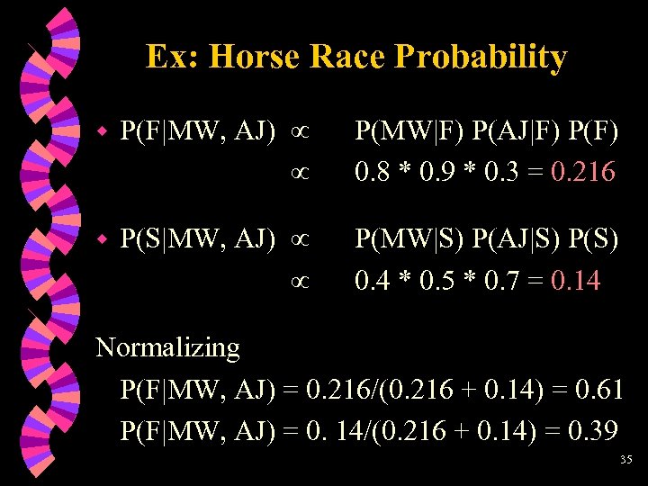
Ex: Horse Race Probability w P(F|MW, AJ) P(MW|F) P(AJ|F) P(F) 0. 8 * 0. 9 * 0. 3 = 0. 216 w P(S|MW, AJ) P(MW|S) P(AJ|S) P(S) 0. 4 * 0. 5 * 0. 7 = 0. 14 Normalizing P(F|MW, AJ) = 0. 216/(0. 216 + 0. 14) = 0. 61 P(F|MW, AJ) = 0. 14/(0. 216 + 0. 14) = 0. 39 35
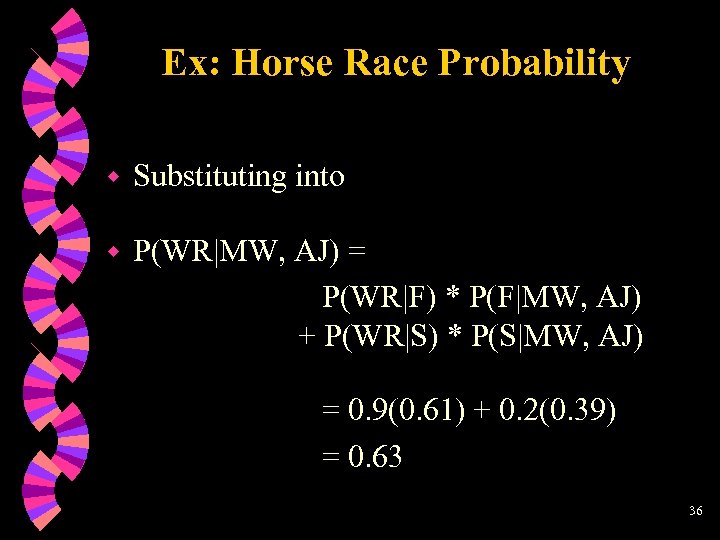
Ex: Horse Race Probability w Substituting into w P(WR|MW, AJ) = P(WR|F) * P(F|MW, AJ) + P(WR|S) * P(S|MW, AJ) = 0. 9(0. 61) + 0. 2(0. 39) = 0. 63 36
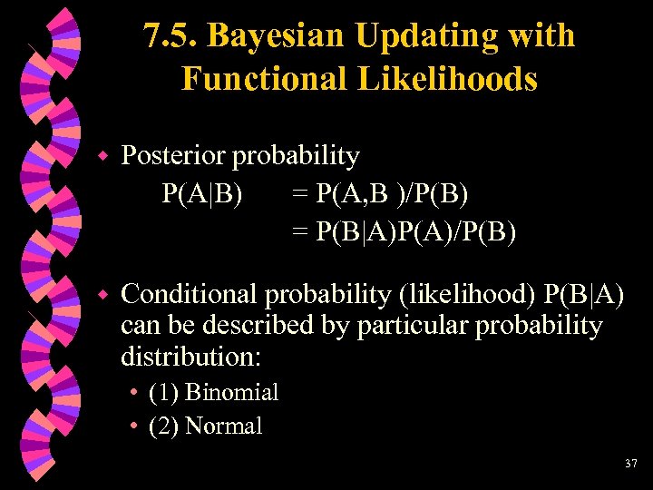
7. 5. Bayesian Updating with Functional Likelihoods w Posterior probability P(A|B) = P(A, B )/P(B) = P(B|A)P(A)/P(B) w Conditional probability (likelihood) P(B|A) can be described by particular probability distribution: • (1) Binomial • (2) Normal 37
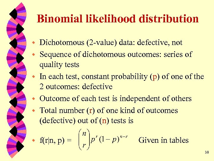
Binomial likelihood distribution w w w Dichotomous (2 -value) data: defective, not Sequence of dichotomous outcomes: series of quality tests In each test, constant probability (p) of one of the 2 outcomes: defective Outcome of each test is independent of others Total number (r) of one kind of outcomes (defective) out of (n) tests is f(r|n, p) = Given in tables 38
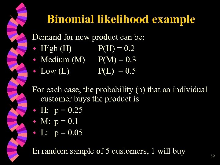
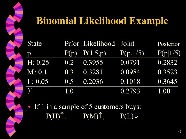
Binomial likelihood example Demand for new product can be: w High (H) P(H) = 0. 2 w Medium (M) P(M) = 0. 3 w Low (L) P(L) = 0. 5 For each case, the probability (p) that an individual customer buys the product is w H: p = 0. 25 w M: p = 0. 1 w L: p = 0. 05 In random sample of 5 customers, 1 will buy 39
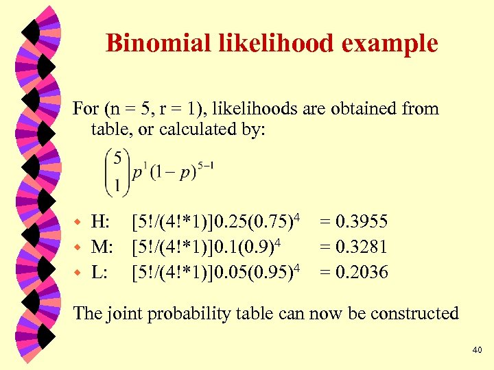
Binomial likelihood example For (n = 5, r = 1), likelihoods are obtained from table, or calculated by: H: [5!/(4!*1)]0. 25(0. 75)4 w M: [5!/(4!*1)]0. 1(0. 9)4 w L: [5!/(4!*1)]0. 05(0. 95)4 w = 0. 3955 = 0. 3281 = 0. 2036 The joint probability table can now be constructed 40
Binomial Likelihood Example State p H: 0. 25 M: 0. 1 L: 0. 05 w Prior P(p) 0. 2 0. 3 0. 5 1. 0 Likelihood P(1|5, p) 0. 3955 0. 3281 0. 2036 Joint P(p, 1/5) 0. 0791 0. 0984 0. 1018 0. 2793 Posterior P(p|1/5) 0. 2832 0. 3523 0. 3645 1. 00 If 1 in a sample of 5 customers buys: P(H) , P(M) , P(L) 41
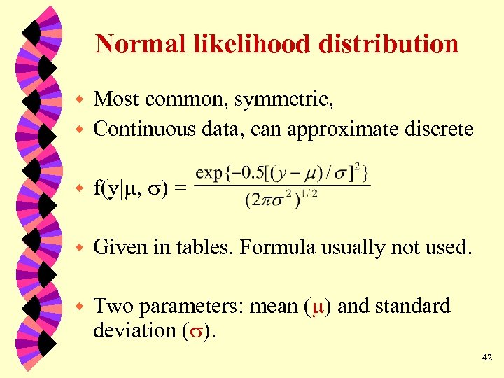
Normal likelihood distribution Most common, symmetric, w Continuous data, can approximate discrete w w f(y| , ) = w Given in tables. Formula usually not used. w Two parameters: mean ( ) and standard deviation ( ). 42
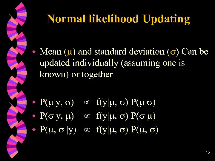
Normal likelihood Updating w Mean ( ) and standard deviation ( ) Can be updated individually (assuming one is known) or together P( |y, ) f(y| , ) P( | ) w P( , |y) f(y| , ) P( , ) w 43
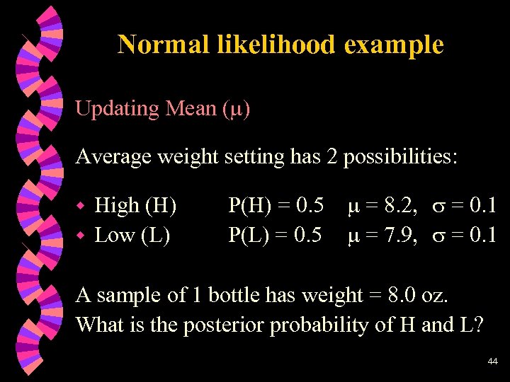
Normal likelihood example Updating Mean ( ) Average weight setting has 2 possibilities: High (H) w Low (L) w P(H) = 0. 5 = 8. 2, = 0. 1 P(L) = 0. 5 = 7. 9, = 0. 1 A sample of 1 bottle has weight = 8. 0 oz. What is the posterior probability of H and L? 44
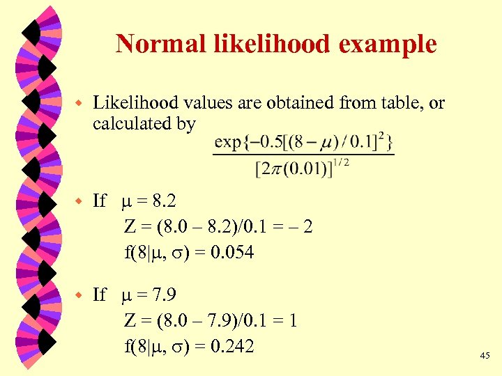
Normal likelihood example w Likelihood values are obtained from table, or calculated by w If = 8. 2 Z = (8. 0 – 8. 2)/0. 1 = – 2 f(8| , ) = 0. 054 w If = 7. 9 Z = (8. 0 – 7. 9)/0. 1 = 1 f(8| , ) = 0. 242 45
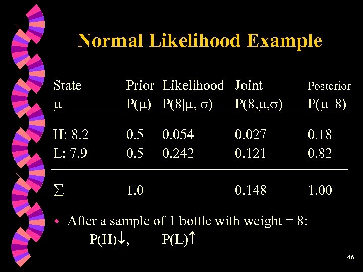
Normal Likelihood Example State Prior Likelihood Joint P( ) P(8| , ) P(8, , ) Posterior H: 8. 2 L: 7. 9 0. 5 0. 027 0. 121 0. 18 0. 82 1. 0 0. 148 1. 00 w 0. 054 0. 242 P( |8) After a sample of 1 bottle with weight = 8: P(H) , P(L) 46
01cd0dd08b533bc63ee04769d3282d36.ppt