1 Chapter 3 — Classical Model INTERNATIONAL

1 Chapter 3 -- Classical Model • INTERNATIONAL ECONOMICS, ECO 486 • Display your name card

2 Learning Objectives • Understand five more assumptions • Determine and understand comparative and absolute advantage • Find international trade equilibrium • Explain gains from trade • Derive range of wages that will permit trade

3 Learning Objectives • Understand five more assumptions • Determine and understand comparative and absolute advantage • Find international trade equilibrium • Explain gains from trade • Derive range of wages that will permit trade

4 Assumption #8 • Factors of production cannot move between countries

5 Assumption #9 • There are no barriers to trade in goods.

6 Assumption #10 • Exports must pay for imports • Assumptions 8 -10 apply to both the Classical and HO Models • Assumptions 11 & 12 apply only to Classical Model

7 Assumption #11 • Labor is the only relevant factor of production in terms of productivity analysis or costs of production.

8 Assumption #12 • Production exhibits constant returns to scale, CRS, between labor and output.

9 CRS Implies Linear PPF • See Figure 3. 1, page 68

10 Autarky • See Figure 3. 2, page 69 • Given perfect competition,

11 Autarky • See Figure 3. 2, page 69 • Given perfect competition, – P = MC – Autarky price of S equals slope of PPF – Resource payments correspond to their productivity

12 Learning Objectives • Understand five more assumptions • Determine and understand comparative and absolute advantage • Find international trade equilibrium • Explain gains from trade • Derive range of wages that will permit trade

13 Absolute Advantage • Compare one good across countries. • Country with lower labor input has an absolute advantage in that good.

14 Comparative Advantage • Calculate opportunity costs. • Compare one good across countries. • Country with lower opportunity cost has a comparative advantage in that good.

15 Which Advantage? • Absolute advantage is a special case. • Comparative advantage is the general case.

16 Learning Objectives • Understand five more assumptions • Determine and understand comparative and absolute advantage • Find international trade equilibrium • Explain gains from trade • Derive range of wages that will permit trade

17 Terms of Trade • Once trade begins, an international equilibrium results • Results in one world price for a good

18 Terms of Trade • Once trade begins, an international equilibrium results • Results in one world price for a good – called the terms of trade – between the two autarky prices – determined by reciprocal demand

19 International Trade Equilibrium • See Figure 3. 3, page 71 • Complete specialization in Comparative Advantage good • CIC & To. T tangent at consumption point • Congruent trade triangles imply balanced trade

20 Learning Objectives • Understand five more assumptions • Determine and understand comparative and absolute advantage • Find international trade equilibrium • Explain gains from trade • Derive range of wages that will permit trade

21 Gains From Trade • Higher CIC shows a gain • Measure gains from trade using GDP • Sources of gain:

22 Gains From Trade • Higher CIC shows a gain • Measure gains from trade using GDP • Sources of gain: – production (gains from specialization) – consumption (To. T price lower than autarky)

23 Learning Objectives • Understand five more assumptions • Determine and understand comparative and absolute advantage • Find international trade equilibrium • Explain gains from trade • Derive range of wages that will permit trade

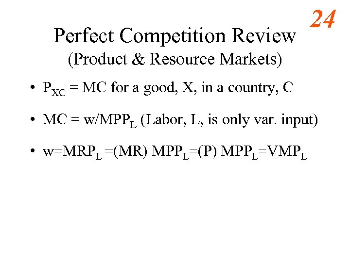Perfect Competition Review 24 (Product & Resource Markets) • PXC = MC for a good, X, in a country, C • MC = w/MPPL (Labor, L, is only var. input) • w=MRPL =(MR) MPPL=(P) MPPL=VMPL

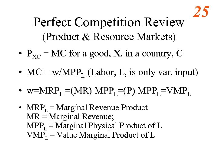Perfect Competition Review 25 (Product & Resource Markets) • PXC = MC for a good, X, in a country, C • MC = w/MPPL (Labor, L, is only var. input) • w=MRPL =(MR) MPPL=(P) MPPL=VMPL • MRPL = Marginal Revenue Product MR = Marginal Revenue; MPPL = Marginal Physical Product of L VMPL = Value Marginal Product of L

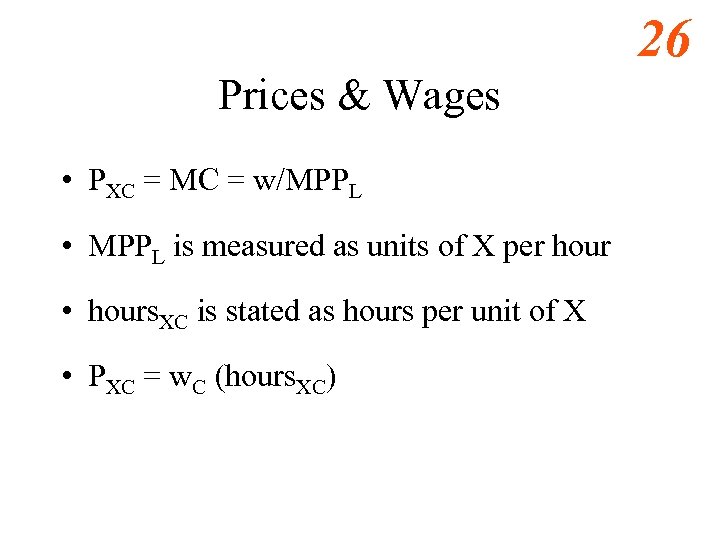26 Prices & Wages • PXC = MC = w/MPPL • MPPL is measured as units of X per hour • hours. XC is stated as hours per unit of X • PXC = w. C (hours. XC)

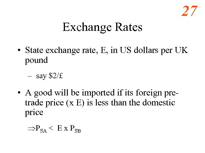27 Exchange Rates • State exchange rate, E, in US dollars per UK pound – say $2/£ • A good will be imported if its foreign pretrade price (x E) is less than the domestic price ÞPSA < E x PSB

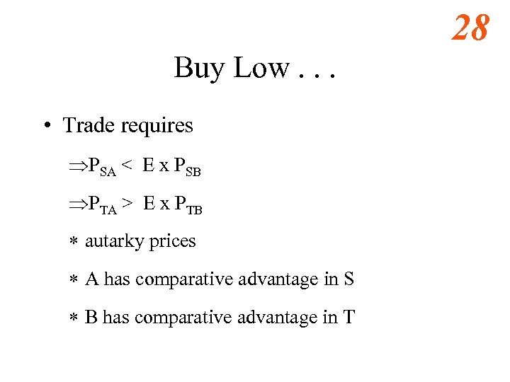28 Buy Low. . . • Trade requires ÞPSA < E x PSB ÞPTA > E x PTB * autarky prices * A has comparative advantage in S * B has comparative advantage in T

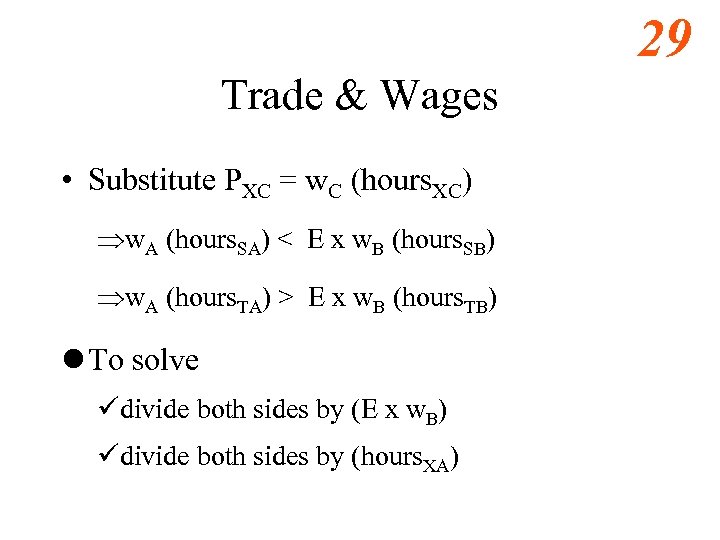29 Trade & Wages • Substitute PXC = w. C (hours. XC) Þw. A (hours. SA) < E x w. B (hours. SB) Þw. A (hours. TA) > E x w. B (hours. TB) l To solve üdivide both sides by (E x w. B) üdivide both sides by (hours. XA)

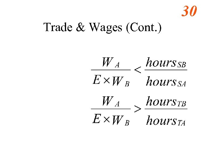30 Trade & Wages (Cont. )

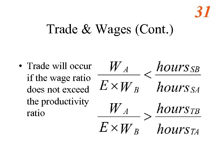31 Trade & Wages (Cont. ) • Trade will occur if the wage ratio does not exceed the productivity ratio

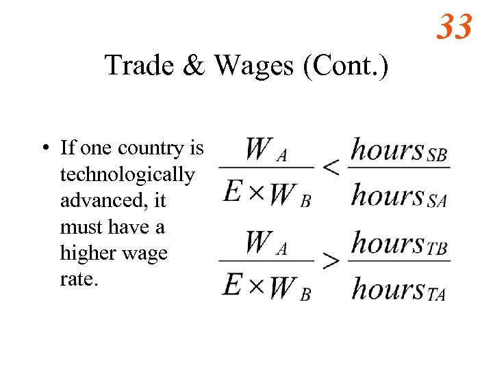33 Trade & Wages (Cont. ) • If one country is technologically advanced, it must have a higher wage rate.

34 Losing Comparative Advantage • If the wage ratio exceeds the productivity ratio, trade will not occur • If a currency is overvalued (say $1/£ instead of $2/£), both goods may be cheaper in one country

35 Review Homework

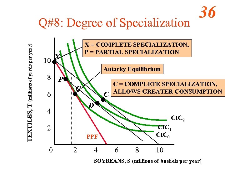TEXTILES, T (millions of yards per year) Q#8: Degree of Specialization 36 X = COMPLETE SPECIALIZATION, P = PARTIAL SPECIALIZATION 10 X Autarky Equilibrium 8 6 P G C C = COMPLETE SPECIALIZATION, ALLOWS GREATER CONSUMPTION D 4 CIC 2 CIC 1 CIC 0 2 PPF 0 2 4 6 8 10 SOYBEANS, S (millions of bushels per year)

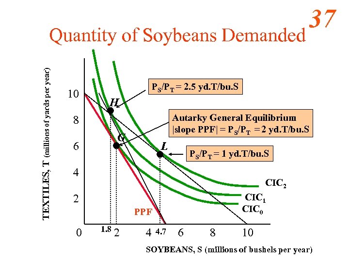TEXTILES, T (millions of yards per year) Quantity of Soybeans Demanded 10 PS/PT = 2. 5 yd. T/bu. S H Autarky General Equilibrium |slope PPF| = PS/PT = 2 yd. T/bu. S 8 G 6 L PS/PT = 1 yd. T/bu. S 4 CIC 2 CIC 1 CIC 0 2 PPF 0 37 1. 8 2 4 4. 7 6 8 10 SOYBEANS, S (millions of bushels per year)