1 CE 530 Molecular Simulation Lecture 25 Efficiencies

1 CE 530 Molecular Simulation Lecture 25 Efficiencies and Parallel Methods David A. Kofke Department of Chemical Engineering SUNY Buffalo kofke@eng. buffalo. edu

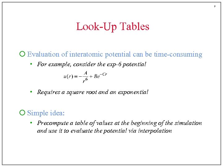2 Look-Up Tables ¡ Evaluation of interatomic potential can be time-consuming • For example, consider the exp-6 potential • Requires a square root and an exponential ¡ Simple idea: • Precompute a table of values at the beginning of the simulation and use it to evaluate the potential via interpolation

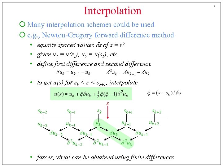Interpolation ¡ Many interpolation schemes could be used ¡ e. g. , Newton-Gregory forward difference method • equally spaced values ds of s = r 2 • given u 1 = u(s 1), u 2 = u(s 2), etc. • define first difference and second difference • to get u(s) for sk < sk+1, interpolate • forces, virial can be obtained using finite differences 3

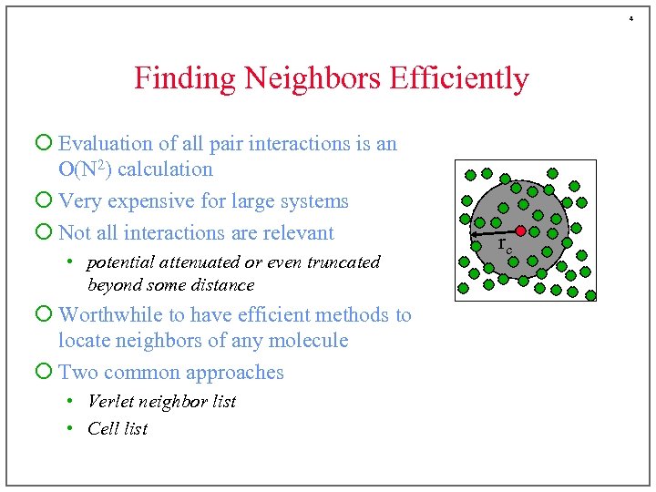4 Finding Neighbors Efficiently ¡ Evaluation of all pair interactions is an O(N 2) calculation ¡ Very expensive for large systems ¡ Not all interactions are relevant • potential attenuated or even truncated beyond some distance ¡ Worthwhile to have efficient methods to locate neighbors of any molecule ¡ Two common approaches • Verlet neighbor list • Cell list rc

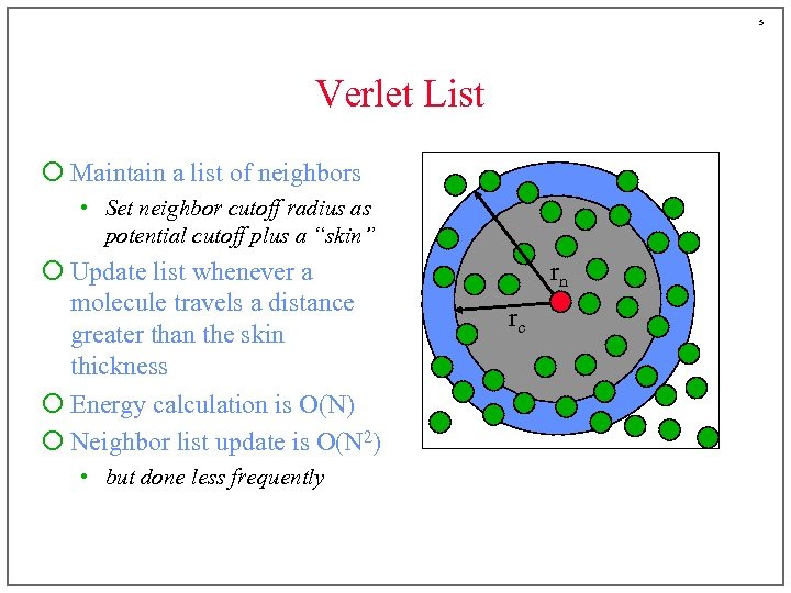5 Verlet List ¡ Maintain a list of neighbors • Set neighbor cutoff radius as potential cutoff plus a “skin” ¡ Update list whenever a molecule travels a distance greater than the skin thickness ¡ Energy calculation is O(N) ¡ Neighbor list update is O(N 2) • but done less frequently rn rc

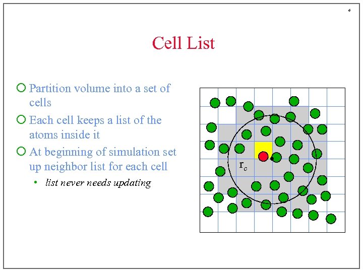6 Cell List ¡ Partition volume into a set of cells ¡ Each cell keeps a list of the atoms inside it ¡ At beginning of simulation set up neighbor list for each cell • list never needs updating rc

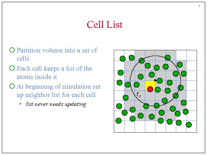7 Cell List ¡ Partition volume into a set of cells ¡ Each cell keeps a list of the atoms inside it ¡ At beginning of simulation set up neighbor list for each cell • list never needs updating rc

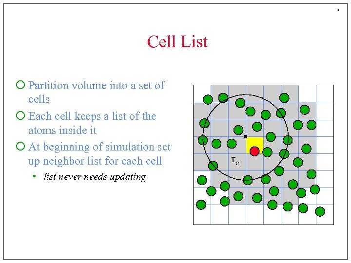8 Cell List ¡ Partition volume into a set of cells ¡ Each cell keeps a list of the atoms inside it ¡ At beginning of simulation set up neighbor list for each cell • list never needs updating rc

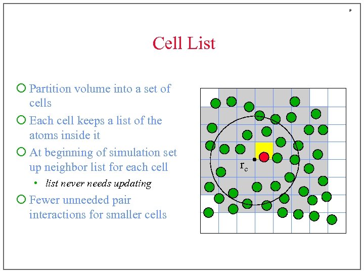9 Cell List ¡ Partition volume into a set of cells ¡ Each cell keeps a list of the atoms inside it ¡ At beginning of simulation set up neighbor list for each cell • list never needs updating ¡ Fewer unneeded pair interactions for smaller cells rc

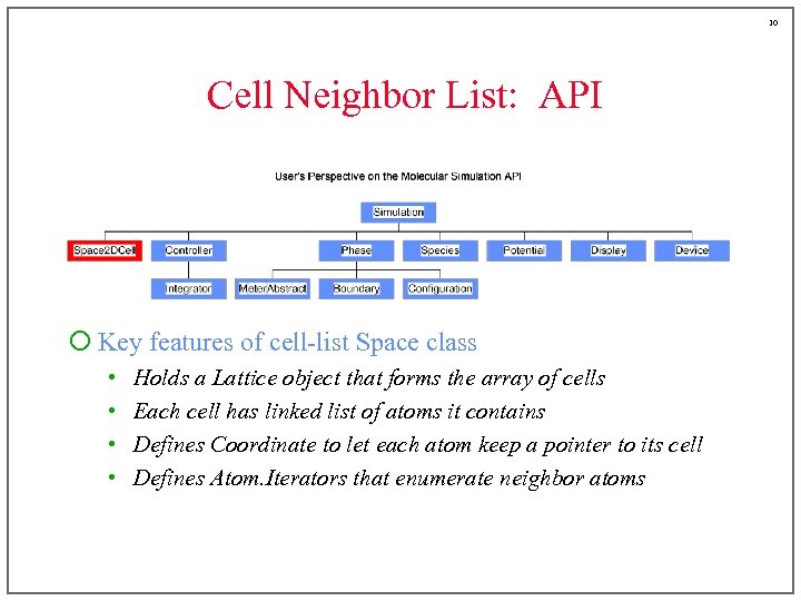10 Cell Neighbor List: API ¡ Key features of cell-list Space class • • Holds a Lattice object that forms the array of cells Each cell has linked list of atoms it contains Defines Coordinate to let each atom keep a pointer to its cell Defines Atom. Iterators that enumerate neighbor atoms

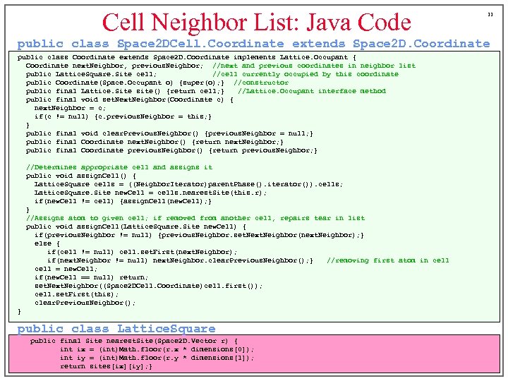Cell Neighbor List: Java Code 11 public class Space 2 DCell. Coordinate extends Space 2 D. Coordinate public class Coordinate extends Space 2 D. Coordinate implements Lattice. Occupant { Coordinate next. Neighbor, previous. Neighbor; //next and previous coordinates in neighbor list public Lattice. Square. Site cell; //cell currently occupied by this coordinate public Coordinate(Space. Occupant o) {super(o); } //constructor public final Lattice. Site site() {return cell; } //Lattice. Occupant interface method public final void set. Next. Neighbor(Coordinate c) { next. Neighbor = c; if(c != null) {c. previous. Neighbor = this; } } public final void clear. Previous. Neighbor() {previous. Neighbor = null; } public final Coordinate next. Neighbor() {return next. Neighbor; } public final Coordinate previous. Neighbor() {return previous. Neighbor; } //Determines appropriate cell and assigns it public void assign. Cell() { Lattice. Square cells = ((Neighbor. Iterator)parent. Phase(). iterator()). cells; Lattice. Square. Site new. Cell = cells. nearest. Site(this. r); if(new. Cell != cell) {assign. Cell(new. Cell); } } //Assigns atom to given cell; if removed from another cell, repairs tear in list public void assign. Cell(Lattice. Square. Site new. Cell) { if(previous. Neighbor != null) {previous. Neighbor. set. Next. Neighbor(next. Neighbor); } else { if(cell != null) cell. set. First(next. Neighbor); if(next. Neighbor != null) next. Neighbor. clear. Previous. Neighbor(); } //removing first atom in cell = new. Cell; if(new. Cell == null) return; set. Next. Neighbor((Space 2 DCell. Coordinate)cell. first()); cell. set. First(this); clear. Previous. Neighbor(); } public class Lattice. Square public final Site nearest. Site(Space 2 D. Vector r) { int ix = (int)Math. floor(r. x * dimensions[0]); int iy = (int)Math. floor(r. y * dimensions[1]); return sites[ix][iy]; }

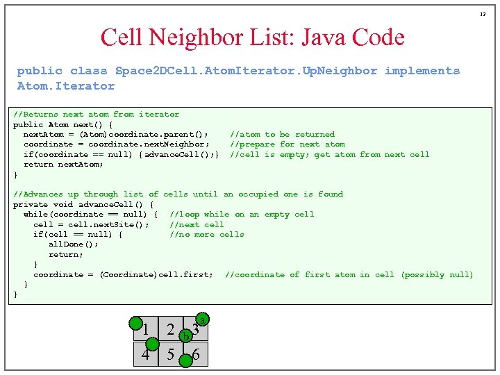12 Cell Neighbor List: Java Code public class Space 2 DCell. Atom. Iterator. Up. Neighbor implements Atom. Iterator //Returns next atom from iterator public Atom next() { next. Atom = (Atom)coordinate. parent(); coordinate = coordinate. next. Neighbor; if(coordinate == null) { advance. Cell(); } return next. Atom; } //atom to be returned //prepare for next atom //cell is empty; get atom from next cell //Advances up through list of cells until an occupied one is found private void advance. Cell() { while(coordinate == null) { //loop while on an empty cell = cell. next. Site(); //next cell if(cell == null) { //no more cells all. Done(); return; } coordinate = (Coordinate)cell. first; //coordinate of first atom in cell (possibly null) } } a 1 2 b 3 4 5 6

13 Parallelizing Simulation Codes ¡ Two parallelization strategies • Domain decomposition Each processor focuses on fixed region of simulation space (cell) Communication needed only with adjacent-cell processors Enables simulation of very large systems for short times • Replicated data Each processor takes some part in advancing all molecules Communication among all processors required Enables simulation of small systems for longer times

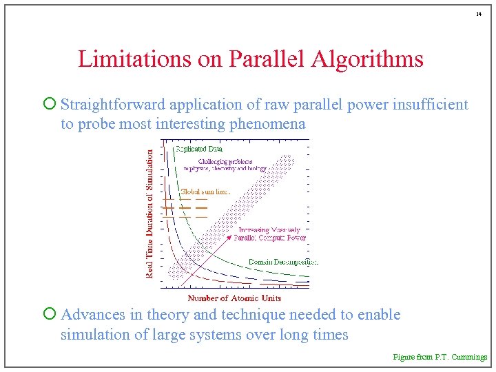14 Limitations on Parallel Algorithms ¡ Straightforward application of raw parallel power insufficient to probe most interesting phenomena ¡ Advances in theory and technique needed to enable simulation of large systems over long times Figure from P. T. Cummings

15 Parallelizing Monte Carlo ¡ Parallel moves in independent regions • moves and range of interactions cannot span large distances ¡ Hybrid Monte Carlo • apply MC as bad MD, and apply MD parallel methods time information lost while introducing limitations of MD ¡ Farming of independent tasks or simulations • equilibration phase is sequential • often a not-too-bad approach ¡ Parallel trials with coupled acceptance • “Esselink” method

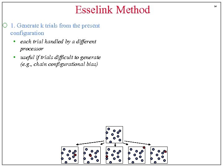Esselink Method ¡ 1. Generate k trials from the present configuration • each trial handled by a different processor • useful if trials difficult to generate (e. g. , chain configurational bias) 16

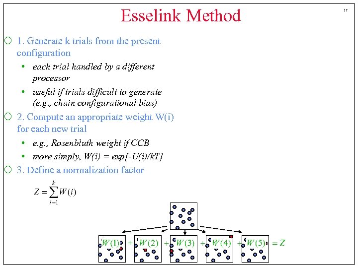Esselink Method ¡ 1. Generate k trials from the present configuration • each trial handled by a different processor • useful if trials difficult to generate (e. g. , chain configurational bias) ¡ 2. Compute an appropriate weight W(i) for each new trial • e. g. , Rosenbluth weight if CCB • more simply, W(i) = exp[-U(i)/k. T] ¡ 3. Define a normalization factor 17

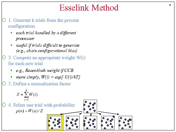Esselink Method ¡ 1. Generate k trials from the present configuration • each trial handled by a different processor • useful if trials difficult to generate (e. g. , chain configurational bias) ¡ 2. Compute an appropriate weight W(i) for each new trial • e. g. , Rosenbluth weight if CCB • more simply, W(i) = exp[-U(i)/k. T] ¡ 3. Define a normalization factor ¡ 4. Select one trial with probability 18

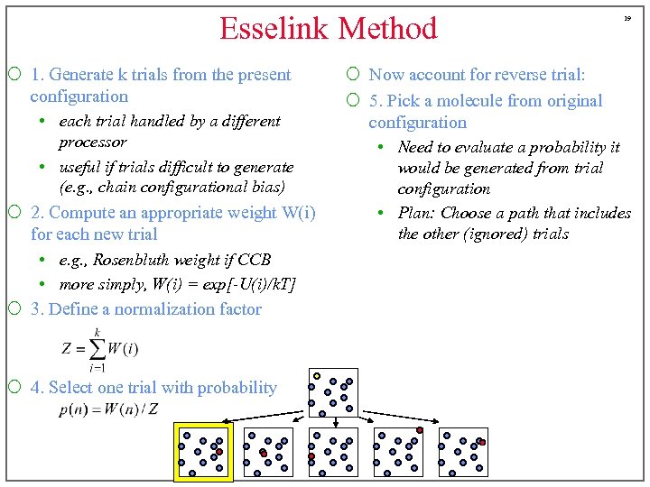Esselink Method ¡ 1. Generate k trials from the present configuration • each trial handled by a different processor • useful if trials difficult to generate (e. g. , chain configurational bias) ¡ 2. Compute an appropriate weight W(i) for each new trial • e. g. , Rosenbluth weight if CCB • more simply, W(i) = exp[-U(i)/k. T] ¡ 3. Define a normalization factor ¡ 4. Select one trial with probability 19 ¡ Now account for reverse trial: ¡ 5. Pick a molecule from original configuration • Need to evaluate a probability it would be generated from trial configuration • Plan: Choose a path that includes the other (ignored) trials

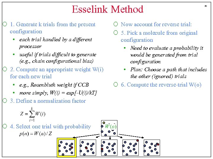Esselink Method ¡ 1. Generate k trials from the present configuration • each trial handled by a different processor • useful if trials difficult to generate (e. g. , chain configurational bias) ¡ 2. Compute an appropriate weight W(i) for each new trial • e. g. , Rosenbluth weight if CCB • more simply, W(i) = exp[-U(i)/k. T] ¡ 3. Define a normalization factor ¡ 4. Select one trial with probability 20 ¡ Now account for reverse trial: ¡ 5. Pick a molecule from original configuration • Need to evaluate a probability it would be generated from trial configuration • Plan: Choose a path that includes the other (ignored) trials ¡ 6. Compute the reverse-trial W(o)

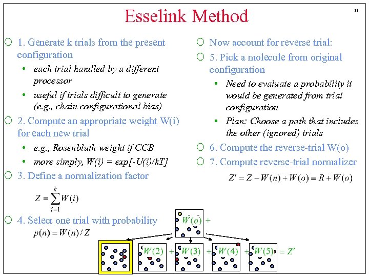Esselink Method ¡ 1. Generate k trials from the present configuration • each trial handled by a different processor • useful if trials difficult to generate (e. g. , chain configurational bias) ¡ 2. Compute an appropriate weight W(i) for each new trial • e. g. , Rosenbluth weight if CCB • more simply, W(i) = exp[-U(i)/k. T] ¡ 3. Define a normalization factor ¡ 4. Select one trial with probability 21 ¡ Now account for reverse trial: ¡ 5. Pick a molecule from original configuration • Need to evaluate a probability it would be generated from trial configuration • Plan: Choose a path that includes the other (ignored) trials ¡ 6. Compute the reverse-trial W(o) ¡ 7. Compute reverse-trial normalizer

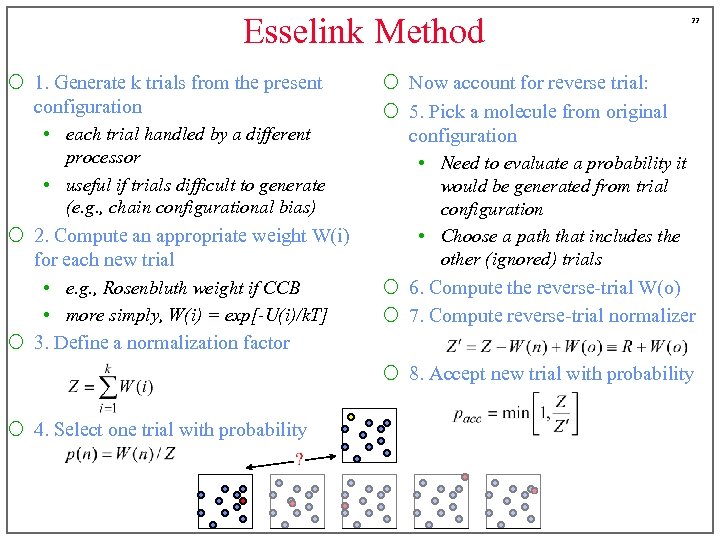Esselink Method ¡ 1. Generate k trials from the present configuration • each trial handled by a different processor • useful if trials difficult to generate (e. g. , chain configurational bias) ¡ 2. Compute an appropriate weight W(i) for each new trial • e. g. , Rosenbluth weight if CCB • more simply, W(i) = exp[-U(i)/k. T] ¡ 3. Define a normalization factor 22 ¡ Now account for reverse trial: ¡ 5. Pick a molecule from original configuration • Need to evaluate a probability it would be generated from trial configuration • Choose a path that includes the other (ignored) trials ¡ 6. Compute the reverse-trial W(o) ¡ 7. Compute reverse-trial normalizer ¡ 8. Accept new trial with probability ¡ 4. Select one trial with probability

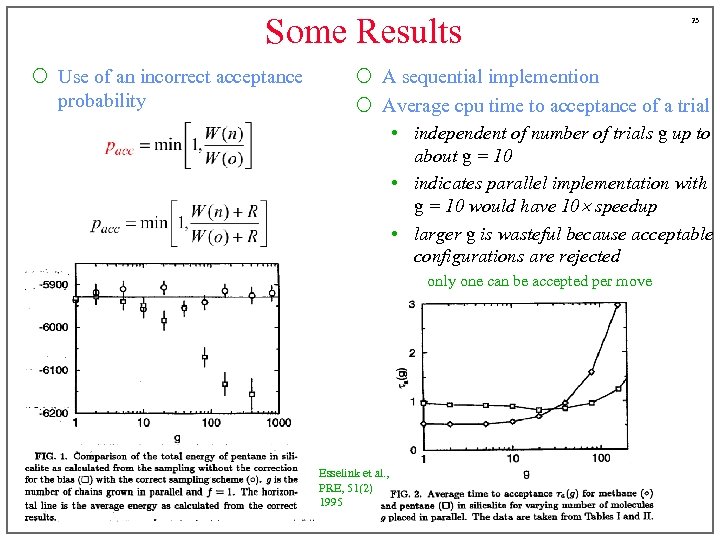Some Results ¡ Use of an incorrect acceptance probability 23 ¡ A sequential implemention ¡ Average cpu time to acceptance of a trial • independent of number of trials g up to about g = 10 • indicates parallel implementation with g = 10 would have 10 speedup • larger g is wasteful because acceptable configurations are rejected only one can be accepted per move Esselink et al. , PRE, 51(2) 1995

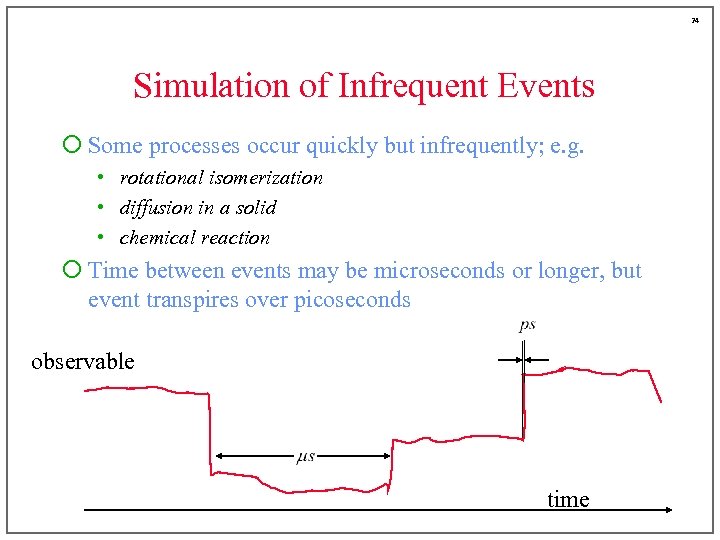24 Simulation of Infrequent Events ¡ Some processes occur quickly but infrequently; e. g. • rotational isomerization • diffusion in a solid • chemical reaction ¡ Time between events may be microseconds or longer, but event transpires over picoseconds observable time

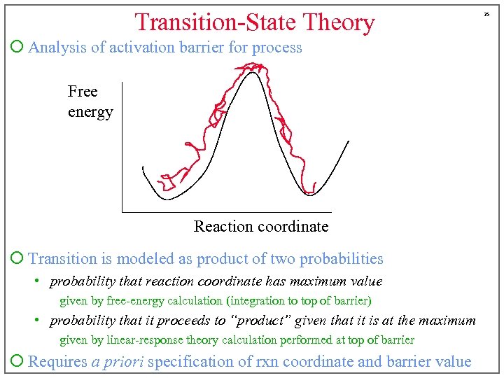Transition-State Theory ¡ Analysis of activation barrier for process Free energy Reaction coordinate ¡ Transition is modeled as product of two probabilities • probability that reaction coordinate has maximum value given by free-energy calculation (integration to top of barrier) • probability that it proceeds to “product” given that it is at the maximum given by linear-response theory calculation performed at top of barrier ¡ Requires a priori specification of rxn coordinate and barrier value 25

26 Parallel Replica Method (Voter’s Method) ¡ Establish several configurations with same coordinates, but different initial momenta ¡ Specify criterion for departure from current “basin” in phase space • e. g. , location of energy minimum evaluate with steepest-descent or conjugate-gradient methods ¡ Perform simulation dynamics in parallel for different initial systems ¡ Continue simulations until one of the replicas is observed to depart its local basin ¡ Advance simulation clock by sum of simulation times of all replicas ¡ Repeat beginning all replicas with coordinates of escaping replica

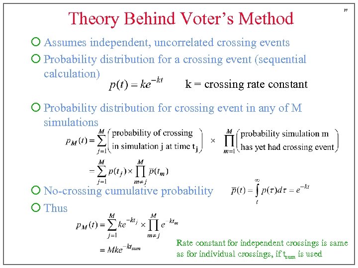Theory Behind Voter’s Method 27 ¡ Assumes independent, uncorrelated crossing events ¡ Probability distribution for a crossing event (sequential calculation) k = crossing rate constant ¡ Probability distribution for crossing event in any of M simulations ¡ No-crossing cumulative probability ¡ Thus Rate constant for independent crossings is same as for individual crossings, if tsum is used

28 Appealing Features of Voter’s Method ¡ No a priori specification of transition path / reaction coordinate required • Works well with multiple (unidentified) transition states • Does not require specification of “product” states ¡ Parallelizes time calculation • “Discarded” simulations are not wasted ¡ Works well in a heterogeneous environment of computing platforms • OK to have processors with different computing power • Parallelization is loosely coupled

29 Summary ¡ Some simple efficiencies to apply to simulations • Table look-up of potentials • Cell lists for identifying neighbors ¡ Parallelization methods • Time parallelization is difficult • Esselink method for parallelization of MC trials • Voter’s method for parallelization of MD simulation of rare events