1 A Primer on Financial Time Series Analysis

1 A Primer on Financial Time Series Analysis Elements of Financial Risk Management Chapter 3 Peter Christoffersen Elements of Financial Risk Management Second Edition © 2012 by Peter Christoffersen

Overview Topics under discussion in this Chapter • • Probability Distributions and Moments The Linear Model Univariate Time Series Models Multivariate Time Series Models Elements of Financial Risk Management Second Edition © 2012 by Peter Christoffersen 2

Common pitfalls encountered while dealing with time series data • Spurious detection of mean-reversion • Spurious regression • Spurious detection of causality Elements of Financial Risk Management Second Edition © 2012 by Peter Christoffersen 3

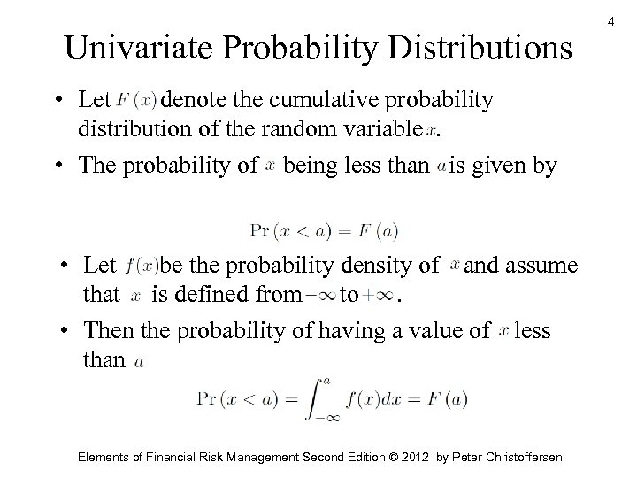Univariate Probability Distributions • Let denote the cumulative probability distribution of the random variable. • The probability of being less than is given by • Let be the probability density of and assume that is defined from to. • Then the probability of having a value of less than Elements of Financial Risk Management Second Edition © 2012 by Peter Christoffersen 4

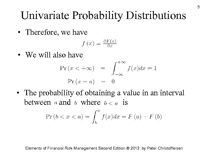Univariate Probability Distributions • Therefore, we have • We will also have • The probability of obtaining a value in an interval between and where is Elements of Financial Risk Management Second Edition © 2012 by Peter Christoffersen 5

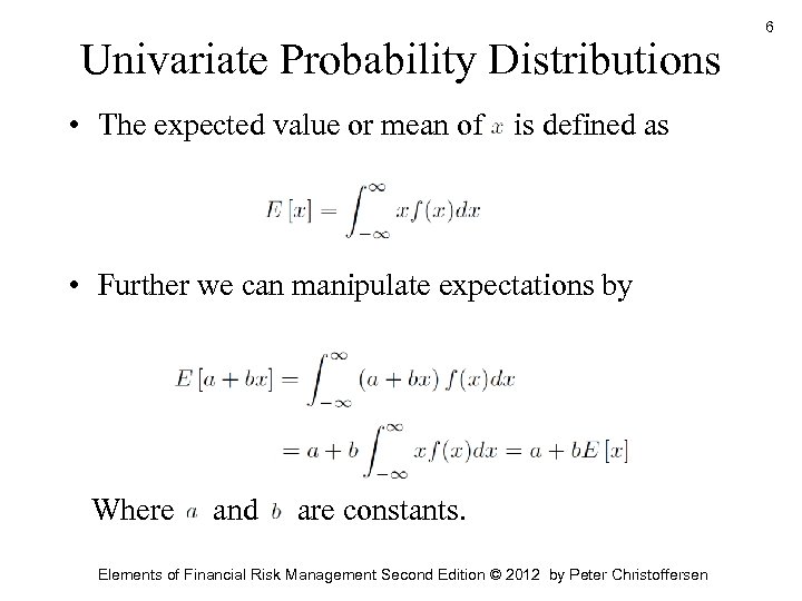Univariate Probability Distributions • The expected value or mean of is defined as • Further we can manipulate expectations by Where and are constants. Elements of Financial Risk Management Second Edition © 2012 by Peter Christoffersen 6

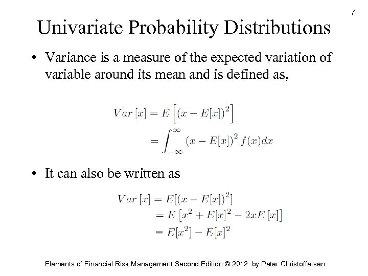Univariate Probability Distributions • Variance is a measure of the expected variation of variable around its mean and is defined as, • It can also be written as Elements of Financial Risk Management Second Edition © 2012 by Peter Christoffersen 7

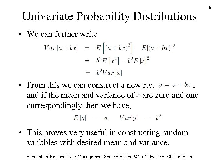Univariate Probability Distributions • We can further write • From this we can construct a new r. v. , and if the mean and variance of are zero and one correspondingly then we have, • This proves very useful in constructing random variables with desired mean and variance. Elements of Financial Risk Management Second Edition © 2012 by Peter Christoffersen 8

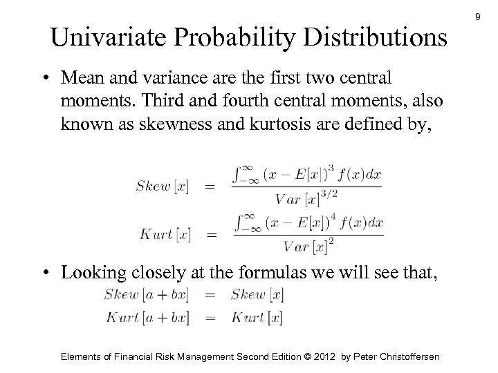Univariate Probability Distributions • Mean and variance are the first two central moments. Third and fourth central moments, also known as skewness and kurtosis are defined by, • Looking closely at the formulas we will see that, Elements of Financial Risk Management Second Edition © 2012 by Peter Christoffersen 9

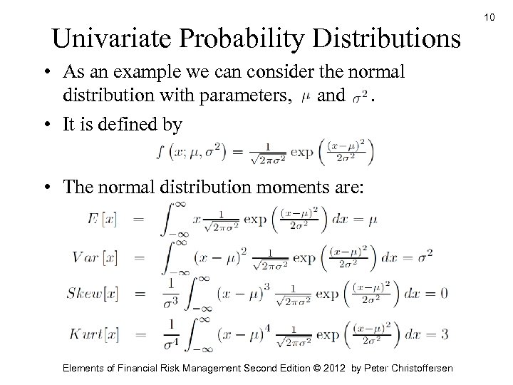Univariate Probability Distributions • As an example we can consider the normal distribution with parameters, and. • It is defined by • The normal distribution moments are: Elements of Financial Risk Management Second Edition © 2012 by Peter Christoffersen 10

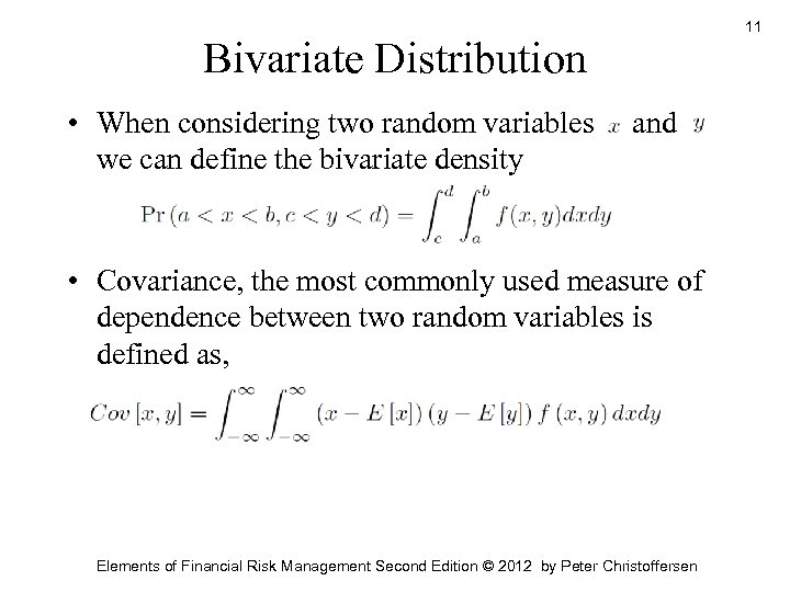11 Bivariate Distribution • When considering two random variables we can define the bivariate density and • Covariance, the most commonly used measure of dependence between two random variables is defined as, Elements of Financial Risk Management Second Edition © 2012 by Peter Christoffersen

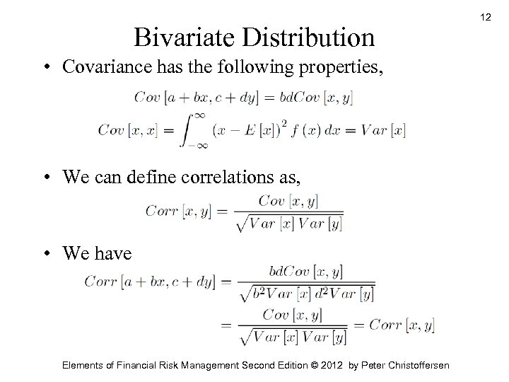Bivariate Distribution • Covariance has the following properties, • We can define correlations as, • We have Elements of Financial Risk Management Second Edition © 2012 by Peter Christoffersen 12

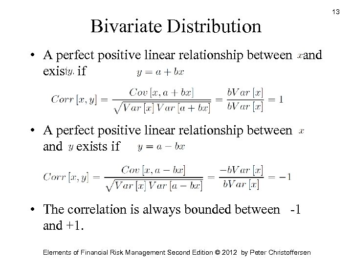Bivariate Distribution • A perfect positive linear relationship between and exists if • The correlation is always bounded between -1 and +1. Elements of Financial Risk Management Second Edition © 2012 by Peter Christoffersen 13

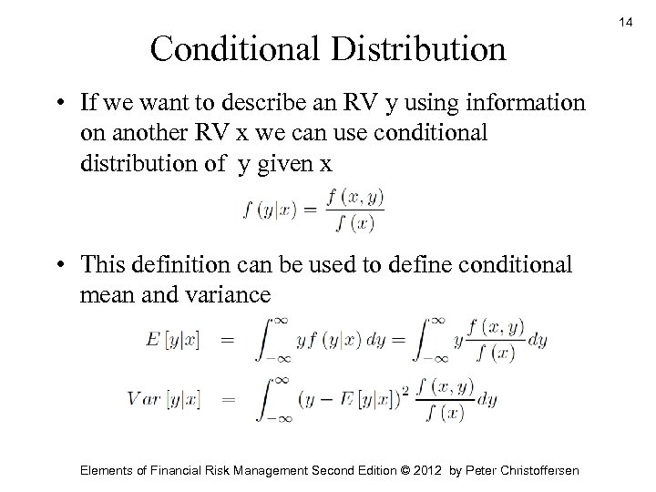Conditional Distribution • If we want to describe an RV y using information on another RV x we can use conditional distribution of y given x • This definition can be used to define conditional mean and variance Elements of Financial Risk Management Second Edition © 2012 by Peter Christoffersen 14

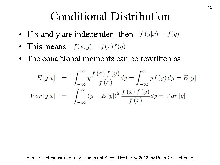Conditional Distribution • If x and y are independent then • This means. • The conditional moments can be rewritten as Elements of Financial Risk Management Second Edition © 2012 by Peter Christoffersen 15

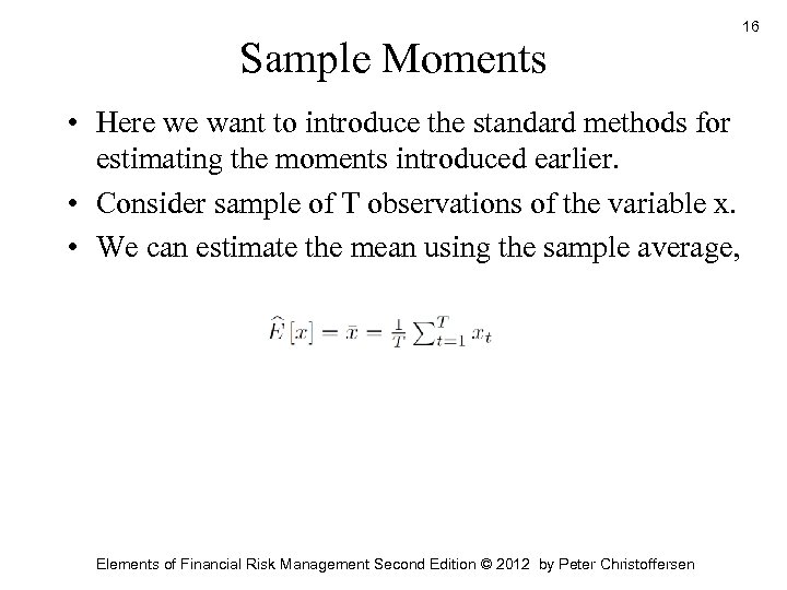Sample Moments • Here we want to introduce the standard methods for estimating the moments introduced earlier. • Consider sample of T observations of the variable x. • We can estimate the mean using the sample average, Elements of Financial Risk Management Second Edition © 2012 by Peter Christoffersen 16

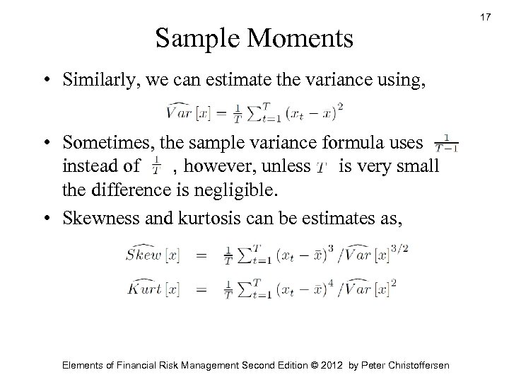Sample Moments • Similarly, we can estimate the variance using, • Sometimes, the sample variance formula uses instead of , however, unless is very small the difference is negligible. • Skewness and kurtosis can be estimates as, Elements of Financial Risk Management Second Edition © 2012 by Peter Christoffersen 17

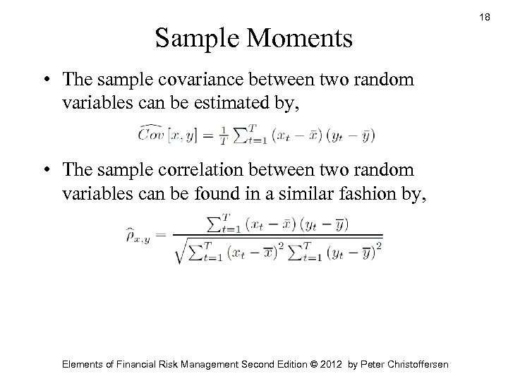Sample Moments • The sample covariance between two random variables can be estimated by, • The sample correlation between two random variables can be found in a similar fashion by, Elements of Financial Risk Management Second Edition © 2012 by Peter Christoffersen 18

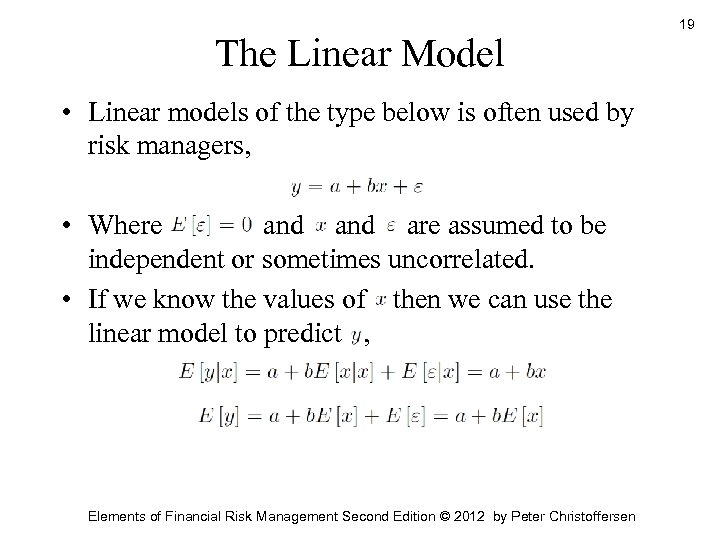The Linear Model • Linear models of the type below is often used by risk managers, • Where and are assumed to be independent or sometimes uncorrelated. • If we know the values of then we can use the linear model to predict , Elements of Financial Risk Management Second Edition © 2012 by Peter Christoffersen 19

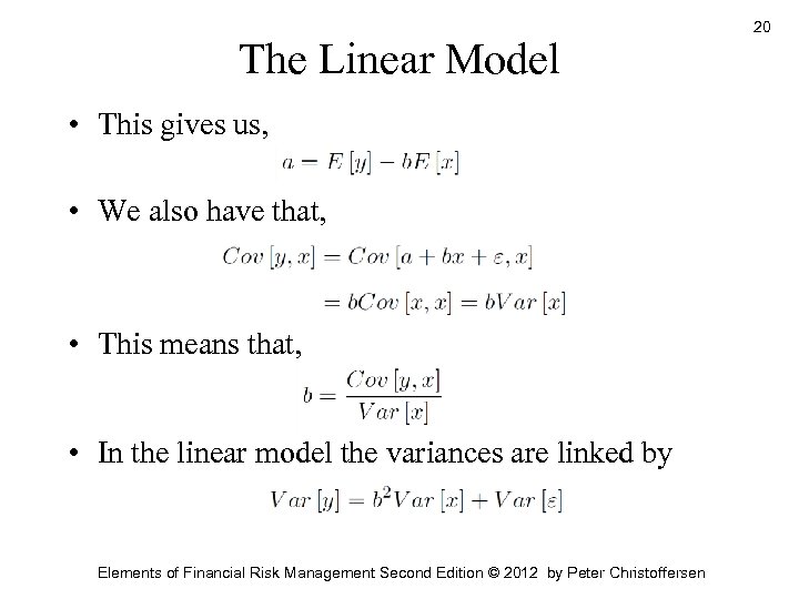The Linear Model • This gives us, • We also have that, • This means that, • In the linear model the variances are linked by Elements of Financial Risk Management Second Edition © 2012 by Peter Christoffersen 20

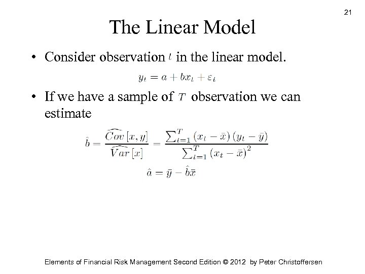The Linear Model • Consider observation in the linear model. • If we have a sample of estimate observation we can Elements of Financial Risk Management Second Edition © 2012 by Peter Christoffersen 21

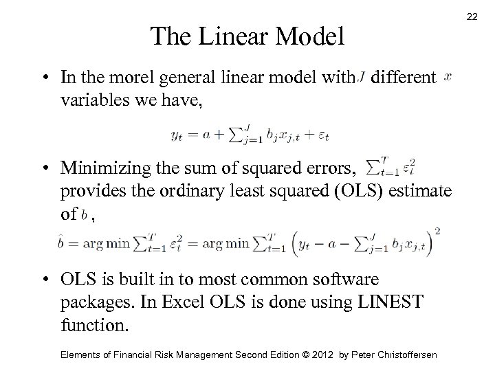The Linear Model • In the morel general linear model with different variables we have, • Minimizing the sum of squared errors, provides the ordinary least squared (OLS) estimate of , • OLS is built in to most common software packages. In Excel OLS is done using LINEST function. Elements of Financial Risk Management Second Edition © 2012 by Peter Christoffersen 22

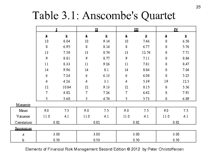
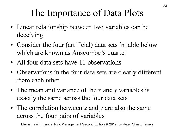The Importance of Data Plots • Linear relationship between two variables can be deceiving • Consider the four (artificial) data sets in table below which are known as Anscombe’s quartet • All four data sets have 11 observations • Observations in the four data sets are clearly different from each other • The mean and variance of the x and y variables is exactly the same across the four data sets • The correlation between x and y are also the same across the four pairs of variables Elements of Financial Risk Management Second Edition © 2012 by Peter Christoffersen 23

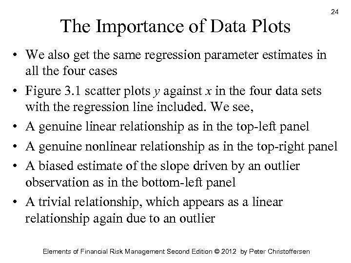The Importance of Data Plots 24 • We also get the same regression parameter estimates in all the four cases • Figure 3. 1 scatter plots y against x in the four data sets with the regression line included. We see, • A genuine linear relationship as in the top-left panel • A genuine nonlinear relationship as in the top-right panel • A biased estimate of the slope driven by an outlier observation as in the bottom-left panel • A trivial relationship, which appears as a linear relationship again due to an outlier Elements of Financial Risk Management Second Edition © 2012 by Peter Christoffersen

25 Table 3. 1: Anscombe's Quartet I II IV x y x y 10 8. 04 10 9. 14 10 7. 46 8 6. 58 8 6. 95 8 8. 14 8 6. 77 8 5. 76 13 7. 58 13 8. 74 13 12. 74 8 7. 71 9 8. 81 9 8. 77 9 7. 11 8 8. 84 11 8. 33 11 9. 26 11 7. 81 8 8. 47 14 9. 96 14 8. 1 14 8. 84 8 7. 04 6 7. 24 6 6. 13 6 6. 08 8 5. 25 4 4. 26 4 3. 1 4 5. 39 19 12. 5 12 10. 84 12 9. 13 12 8. 15 8 5. 56 7 4. 82 7 7. 26 7 6. 42 8 7. 91 5 5. 68 5 4. 74 5 5. 73 8 6. 89 Mean 9. 0 7. 5 Variance 11. 0 4. 1 Moments Correlation 0. 82 a 3. 00 b 0. 50 Regression Elements of Financial Risk Management Second Edition © 2012 by Peter Christoffersen

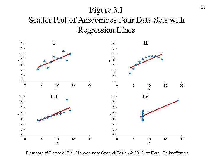Figure 3. 1 Scatter Plot of Anscombes Four Data Sets with Regression Lines I 14 10 8 8 y 12 10 y 12 6 6 4 4 2 2 0 0 5 10 x 15 0 20 0 III 14 5 20 15 20 8 y 10 8 15 12 10 10 x IV 14 12 y II 14 6 6 4 4 2 2 0 0 0 5 10 x 15 20 0 5 10 x Elements of Financial Risk Management Second Edition © 2012 by Peter Christoffersen 26

Univariate Time Series Models • It studies the behavior of a single random variable observed over time • These models forecast the future values of a variable using past and current observations on the same variable Elements of Financial Risk Management Second Edition © 2012 by Peter Christoffersen 27

Autocorrelation • Autocorrelation measures the dependence between the current value of a time series variable and the past value of the same variable. • The autocorrelation for lag is defined as • It captures the linear relationship between today’s value and the value days ago Elements of Financial Risk Management Second Edition © 2012 by Peter Christoffersen 28

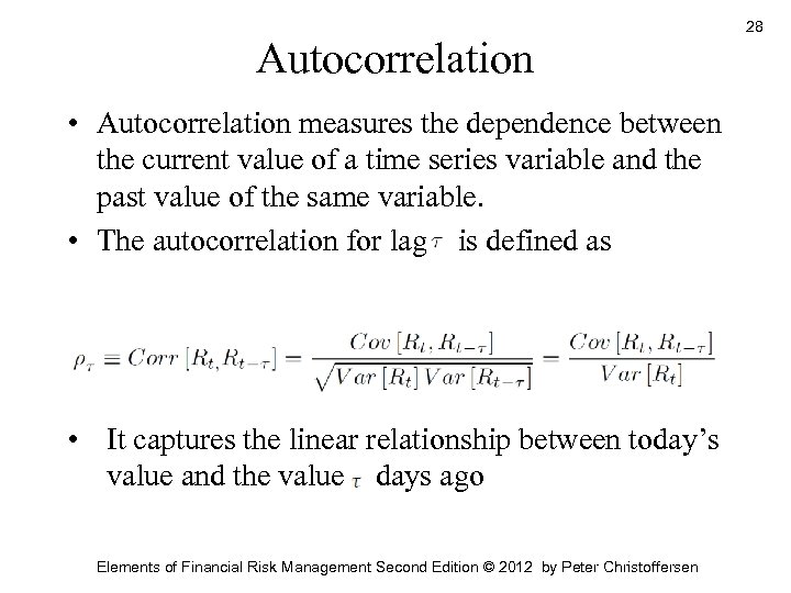
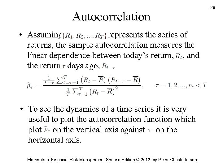Autocorrelation • Assuming represents the series of returns, the sample autocorrelation measures the linear dependence between today’s return, , and the return days ago, • To see the dynamics of a time series it is very useful to plot the autocorrelation function which plot on the vertical axis against on the horizontal axis. Elements of Financial Risk Management Second Edition © 2012 by Peter Christoffersen 29

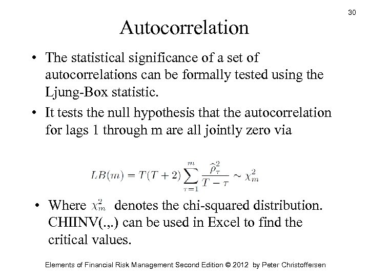Autocorrelation • The statistical significance of a set of autocorrelations can be formally tested using the Ljung-Box statistic. • It tests the null hypothesis that the autocorrelation for lags 1 through m are all jointly zero via • Where denotes the chi-squared distribution. CHIINV(. , . ) can be used in Excel to find the critical values. Elements of Financial Risk Management Second Edition © 2012 by Peter Christoffersen 30

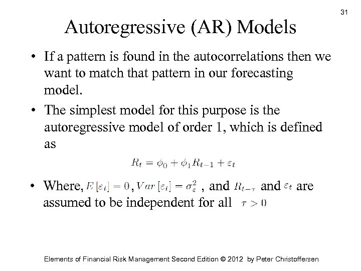Autoregressive (AR) Models • If a pattern is found in the autocorrelations then we want to match that pattern in our forecasting model. • The simplest model for this purpose is the autoregressive model of order 1, which is defined as • Where, , , and assumed to be independent for all and. are Elements of Financial Risk Management Second Edition © 2012 by Peter Christoffersen 31

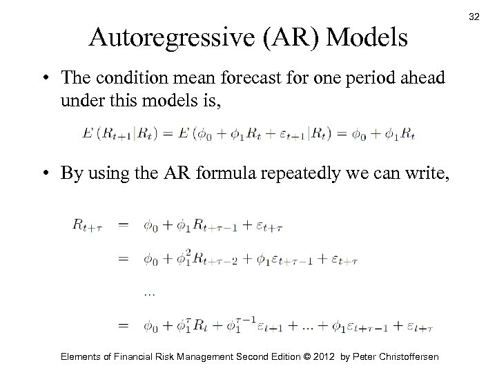Autoregressive (AR) Models • The condition mean forecast for one period ahead under this models is, • By using the AR formula repeatedly we can write, Elements of Financial Risk Management Second Edition © 2012 by Peter Christoffersen 32

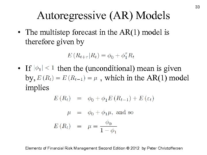Autoregressive (AR) Models • The multistep forecast in the AR(1) model is therefore given by • If by, implies then the (unconditional) mean is given , which in the AR(1) model Elements of Financial Risk Management Second Edition © 2012 by Peter Christoffersen 33

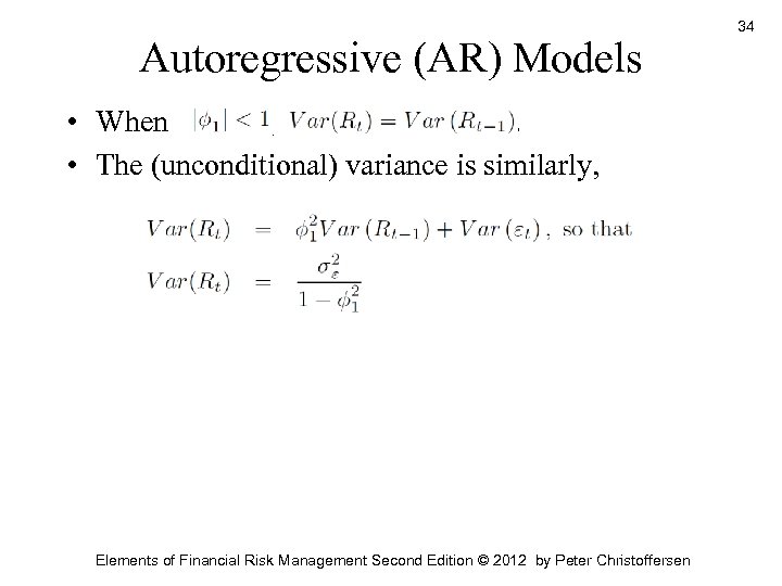Autoregressive (AR) Models • When , . • The (unconditional) variance is similarly, Elements of Financial Risk Management Second Edition © 2012 by Peter Christoffersen 34

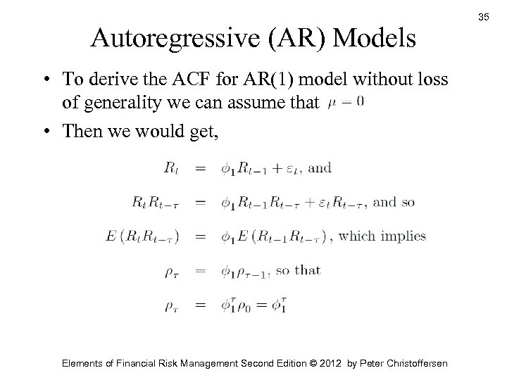Autoregressive (AR) Models • To derive the ACF for AR(1) model without loss of generality we can assume that • Then we would get, Elements of Financial Risk Management Second Edition © 2012 by Peter Christoffersen 35

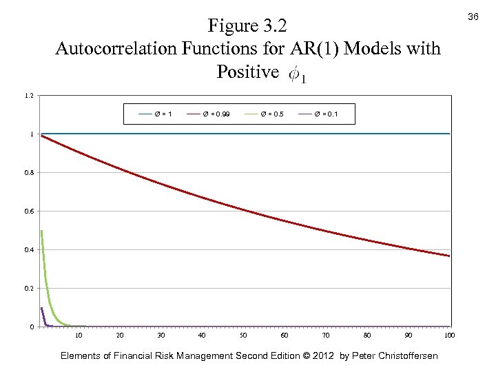36 Figure 3. 2 Autocorrelation Functions for AR(1) Models with Positive 1. 2 Ø=1 Ø = 0. 99 Ø = 0. 5 Ø = 0. 1 1 0. 8 0. 6 0. 4 0. 2 0 10 20 30 40 50 60 70 80 90 Elements of Financial Risk Management Second Edition © 2012 by Peter Christoffersen 100

Autoregressive (AR) Models • Figure 3. 2 shows examples of the ACF in AR(1) models • When <1 then the ACF decays to zero exponentially • The decay is much slower when = 0. 99 than when it is 0. 5 or 0. 1 • When =1 then the ACF is flat at 1. This is the case of a random walk Elements of Financial Risk Management Second Edition © 2012 by Peter Christoffersen 37

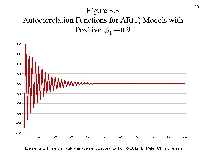Figure 3. 3 Autocorrelation Functions for AR(1) Models with Positive =-0. 9 0. 8 0. 6 0. 4 0. 2 0. 0 -0. 2 -0. 4 -0. 6 -0. 8 -1. 0 10 20 30 40 50 60 70 80 90 Elements of Financial Risk Management Second Edition © 2012 by Peter Christoffersen 100 38

Autoregressive (AR) Models • Figure 3. 3 shows the ACF of an AR(1) when. =-0. 9 • When <0 then the ACF oscillates around zero but it still decays to zero as the lag order increases • The ACFs in Figure 3. 2 are much more common in financial risk management than are the ACFs in Figure 3. 3 Elements of Financial Risk Management Second Edition © 2012 by Peter Christoffersen 39

Autoregressive (AR) Models • The simplest extension to the AR(1) model is the AR(2) model defined as, • The ACF of the AR(2) is • Because for example, • So that, Elements of Financial Risk Management Second Edition © 2012 by Peter Christoffersen 40

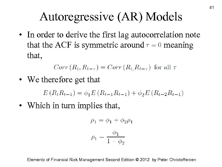Autoregressive (AR) Models • In order to derive the first lag autocorrelation note that the ACF is symmetric around meaning that, • We therefore get that • Which in turn implies that, Elements of Financial Risk Management Second Edition © 2012 by Peter Christoffersen 41

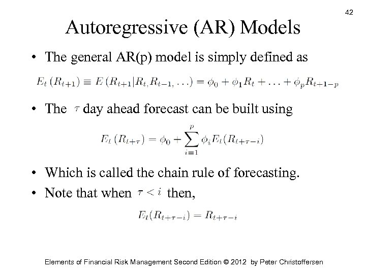Autoregressive (AR) Models • The general AR(p) model is simply defined as • The day ahead forecast can be built using • Which is called the chain rule of forecasting. • Note that when then, Elements of Financial Risk Management Second Edition © 2012 by Peter Christoffersen 42

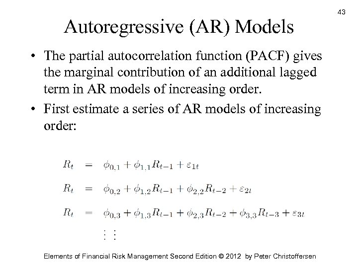Autoregressive (AR) Models • The partial autocorrelation function (PACF) gives the marginal contribution of an additional lagged term in AR models of increasing order. • First estimate a series of AR models of increasing order: Elements of Financial Risk Management Second Edition © 2012 by Peter Christoffersen 43

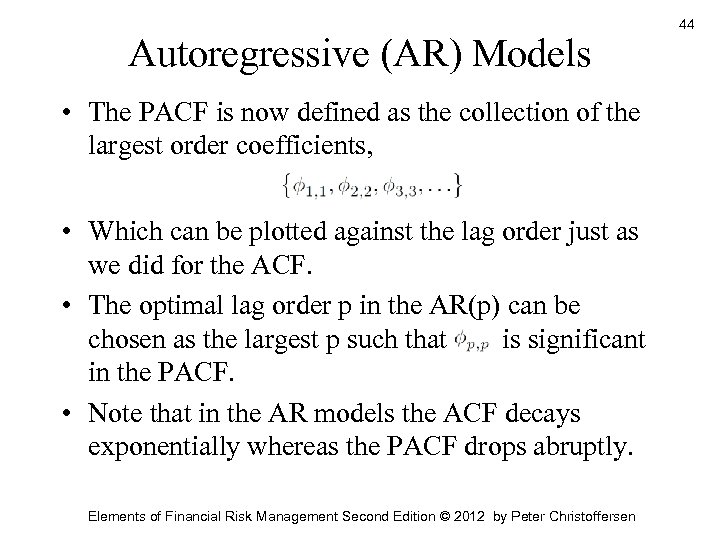Autoregressive (AR) Models • The PACF is now defined as the collection of the largest order coefficients, • Which can be plotted against the lag order just as we did for the ACF. • The optimal lag order p in the AR(p) can be chosen as the largest p such that is significant in the PACF. • Note that in the AR models the ACF decays exponentially whereas the PACF drops abruptly. Elements of Financial Risk Management Second Edition © 2012 by Peter Christoffersen 44

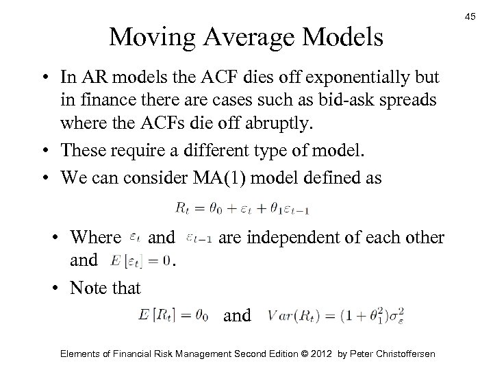Moving Average Models • In AR models the ACF dies off exponentially but in finance there are cases such as bid-ask spreads where the ACFs die off abruptly. • These require a different type of model. • We can consider MA(1) model defined as • Where and. • Note that » are independent of each other and Elements of Financial Risk Management Second Edition © 2012 by Peter Christoffersen 45

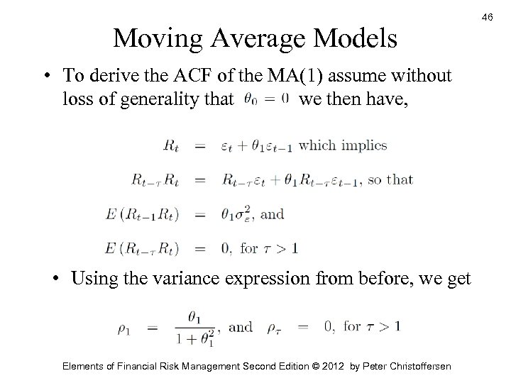Moving Average Models • To derive the ACF of the MA(1) assume without loss of generality that we then have, • Using the variance expression from before, we get Elements of Financial Risk Management Second Edition © 2012 by Peter Christoffersen 46

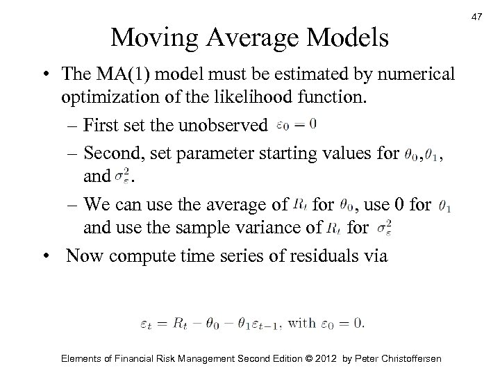Moving Average Models • The MA(1) model must be estimated by numerical optimization of the likelihood function. – First set the unobserved – Second, set parameter starting values for , , and. – We can use the average of for , use 0 for and use the sample variance of for • Now compute time series of residuals via Elements of Financial Risk Management Second Edition © 2012 by Peter Christoffersen 47

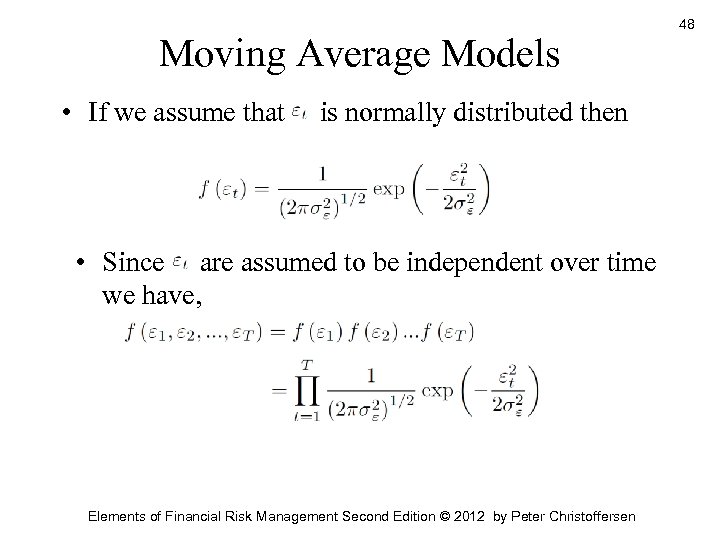Moving Average Models • If we assume that is normally distributed then • Since are assumed to be independent over time we have, Elements of Financial Risk Management Second Edition © 2012 by Peter Christoffersen 48

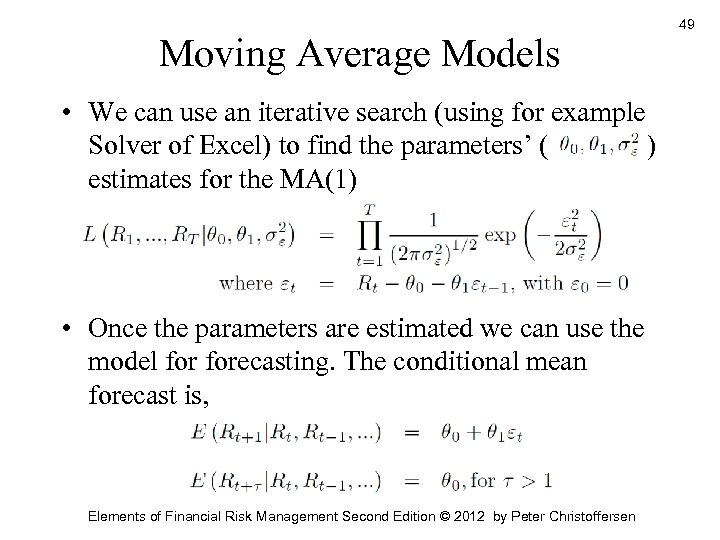Moving Average Models • We can use an iterative search (using for example Solver of Excel) to find the parameters’ ( ) estimates for the MA(1) • Once the parameters are estimated we can use the model forecasting. The conditional mean forecast is, Elements of Financial Risk Management Second Edition © 2012 by Peter Christoffersen 49

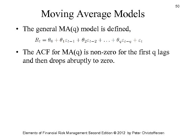Moving Average Models • The general MA(q) model is defined, • The ACF for MA(q) is non-zero for the first q lags and then drops abruptly to zero. Elements of Financial Risk Management Second Edition © 2012 by Peter Christoffersen 50

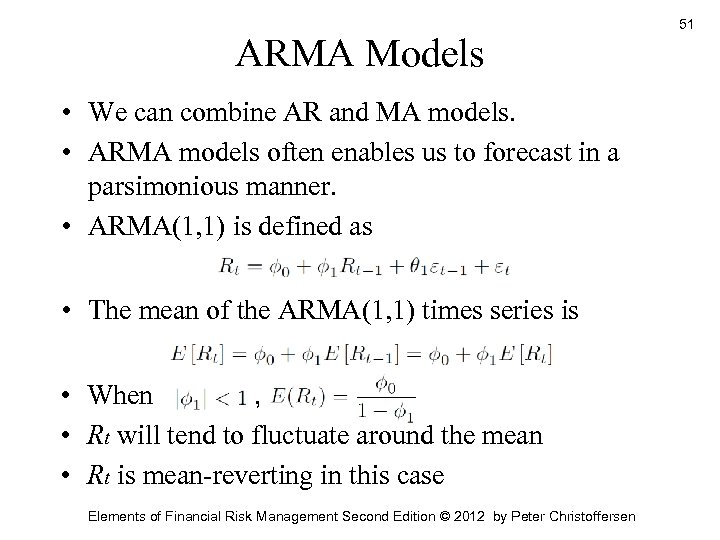ARMA Models • We can combine AR and MA models. • ARMA models often enables us to forecast in a parsimonious manner. • ARMA(1, 1) is defined as • The mean of the ARMA(1, 1) times series is • When , • Rt will tend to fluctuate around the mean • Rt is mean-reverting in this case Elements of Financial Risk Management Second Edition © 2012 by Peter Christoffersen 51

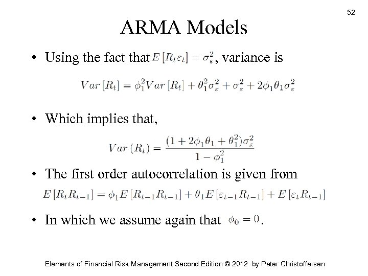52 ARMA Models • Using the fact that , variance is • Which implies that, • The first order autocorrelation is given from • In which we assume again that . Elements of Financial Risk Management Second Edition © 2012 by Peter Christoffersen

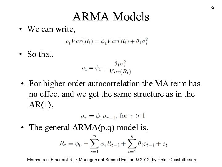ARMA Models • We can write, • So that, • For higher order autocorrelation the MA term has no effect and we get the same structure as in the AR(1), • The general ARMA(p, q) model is, Elements of Financial Risk Management Second Edition © 2012 by Peter Christoffersen 53

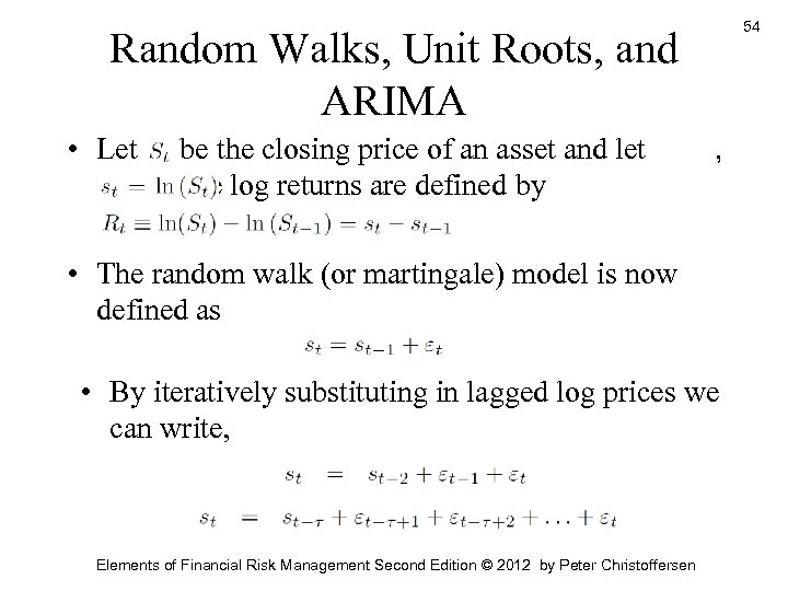54 Random Walks, Unit Roots, and ARIMA • Let , be the closing price of an asset and let so that the log returns are defined by , • The random walk (or martingale) model is now defined as • By iteratively substituting in lagged log prices we can write, Elements of Financial Risk Management Second Edition © 2012 by Peter Christoffersen

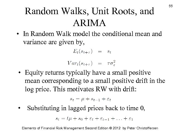Random Walks, Unit Roots, and ARIMA • In Random Walk model the conditional mean and variance are given by, • Equity returns typically have a small positive mean corresponding to a small positive drift in the log price. This motivates RW with drift: • Substituting in lagged prices back to time 0, Elements of Financial Risk Management Second Edition © 2012 by Peter Christoffersen 55

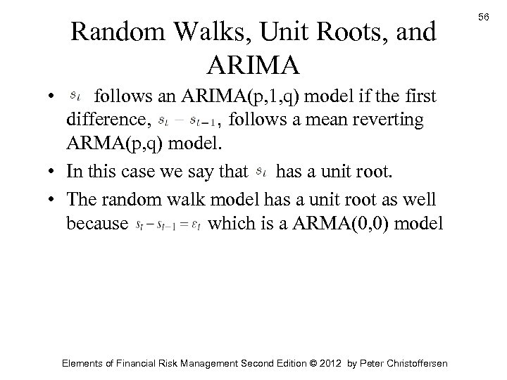Random Walks, Unit Roots, and ARIMA • follows an ARIMA(p, 1, q) model if the first difference, , follows a mean reverting ARMA(p, q) model. • In this case we say that has a unit root. • The random walk model has a unit root as well because which is a ARMA(0, 0) model Elements of Financial Risk Management Second Edition © 2012 by Peter Christoffersen 56

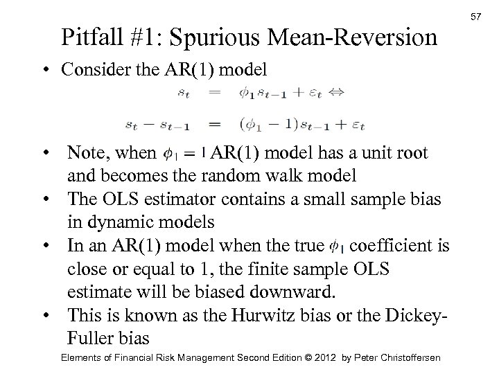Pitfall #1: Spurious Mean-Reversion • Consider the AR(1) model • Note, when , AR(1) model has a unit root and becomes the random walk model • The OLS estimator contains a small sample bias in dynamic models • In an AR(1) model when the true coefficient is close or equal to 1, the finite sample OLS estimate will be biased downward. • This is known as the Hurwitz bias or the Dickey. Fuller bias Elements of Financial Risk Management Second Edition © 2012 by Peter Christoffersen 57

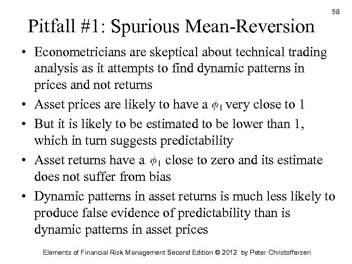Pitfall #1: Spurious Mean-Reversion 58 • Econometricians are skeptical about technical trading analysis as it attempts to find dynamic patterns in prices and not returns • Asset prices are likely to have a very close to 1 • But it is likely to be estimated to be lower than 1, which in turn suggests predictability • Asset returns have a close to zero and its estimate does not suffer from bias • Dynamic patterns in asset returns is much less likely to produce false evidence of predictability than is dynamic patterns in asset prices Elements of Financial Risk Management Second Edition © 2012 by Peter Christoffersen

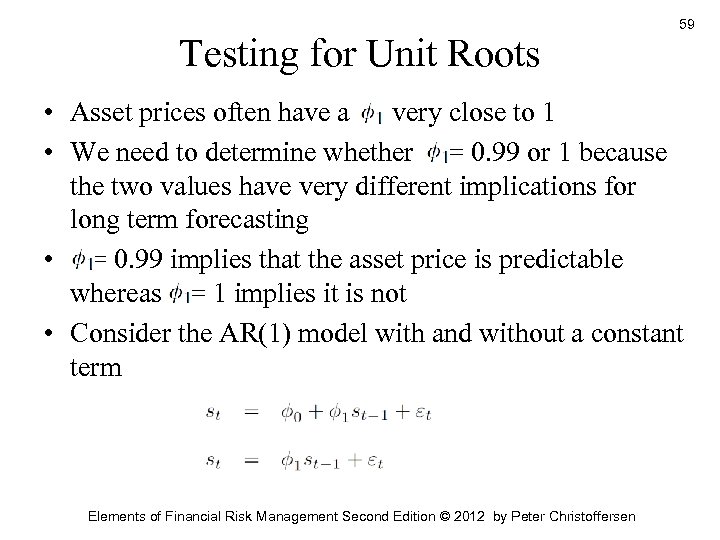Testing for Unit Roots 59 • Asset prices often have a very close to 1 • We need to determine whether = 0. 99 or 1 because the two values have very different implications for long term forecasting • = 0. 99 implies that the asset price is predictable whereas = 1 implies it is not • Consider the AR(1) model with and without a constant term Elements of Financial Risk Management Second Edition © 2012 by Peter Christoffersen

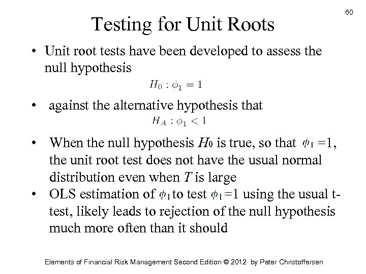Testing for Unit Roots • Unit root tests have been developed to assess the null hypothesis • against the alternative hypothesis that • When the null hypothesis H 0 is true, so that =1, the unit root test does not have the usual normal distribution even when T is large • OLS estimation of to test =1 using the usual ttest, likely leads to rejection of the null hypothesis much more often than it should Elements of Financial Risk Management Second Edition © 2012 by Peter Christoffersen 60

Multivariate Time Series Models • Multivariate time series analysis consider risk models with multiple related risk factors or models with many assets • This section will introduce the following topics: Ø Time series regressions Ø Spurious relationships Ø Cointegration Ø Cross correlations Ø Vector autoregressions Ø Spurious causality Elements of Financial Risk Management Second Edition © 2012 by Peter Christoffersen 61

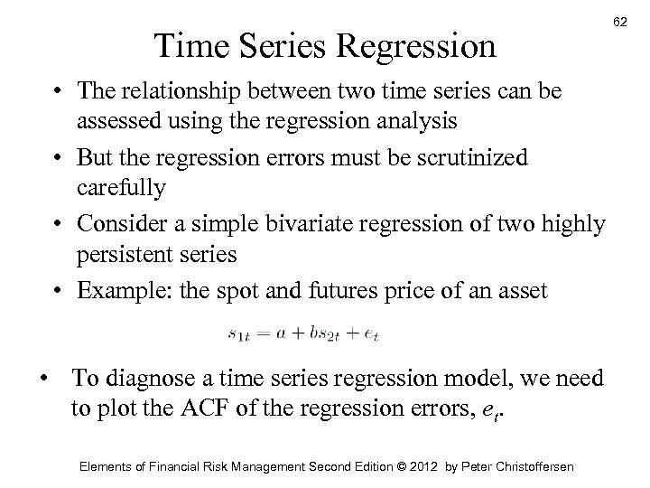Time Series Regression • The relationship between two time series can be assessed using the regression analysis • But the regression errors must be scrutinized carefully • Consider a simple bivariate regression of two highly persistent series • Example: the spot and futures price of an asset • To diagnose a time series regression model, we need to plot the ACF of the regression errors, et. Elements of Financial Risk Management Second Edition © 2012 by Peter Christoffersen 62

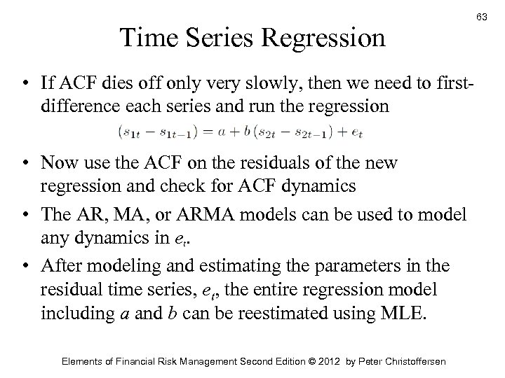Time Series Regression • If ACF dies off only very slowly, then we need to firstdifference each series and run the regression • Now use the ACF on the residuals of the new regression and check for ACF dynamics • The AR, MA, or ARMA models can be used to model any dynamics in et. • After modeling and estimating the parameters in the residual time series, et, the entire regression model including a and b can be reestimated using MLE. Elements of Financial Risk Management Second Edition © 2012 by Peter Christoffersen 63

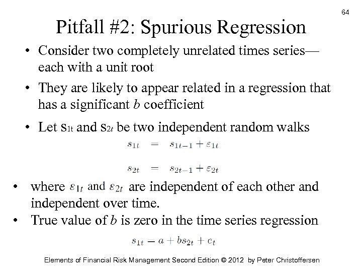Pitfall #2: Spurious Regression • Consider two completely unrelated times series— each with a unit root • They are likely to appear related in a regression that has a significant b coefficient • Let s 1 t and s 2 t be two independent random walks • where are independent of each other and independent over time. • True value of b is zero in the time series regression Elements of Financial Risk Management Second Edition © 2012 by Peter Christoffersen 64

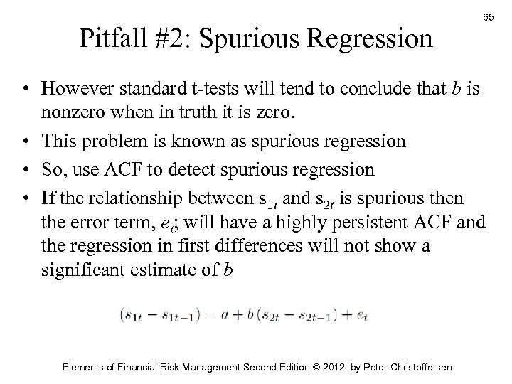Pitfall #2: Spurious Regression 65 • However standard t-tests will tend to conclude that b is nonzero when in truth it is zero. • This problem is known as spurious regression • So, use ACF to detect spurious regression • If the relationship between s 1 t and s 2 t is spurious then the error term, et; will have a highly persistent ACF and the regression in first differences will not show a significant estimate of b Elements of Financial Risk Management Second Edition © 2012 by Peter Christoffersen

Cointegration • Relationships between variables with unit roots are not always spurious. • A variable with a unit root is also called integrated • If two variables that are both integrated have a linear combination with no unit root then we say they are cointegrated. • Examples: long-run consumption and production in an economy • The spot and the futures price of an asset that are related via a no-arbitrage condition. Elements of Financial Risk Management Second Edition © 2012 by Peter Christoffersen 66

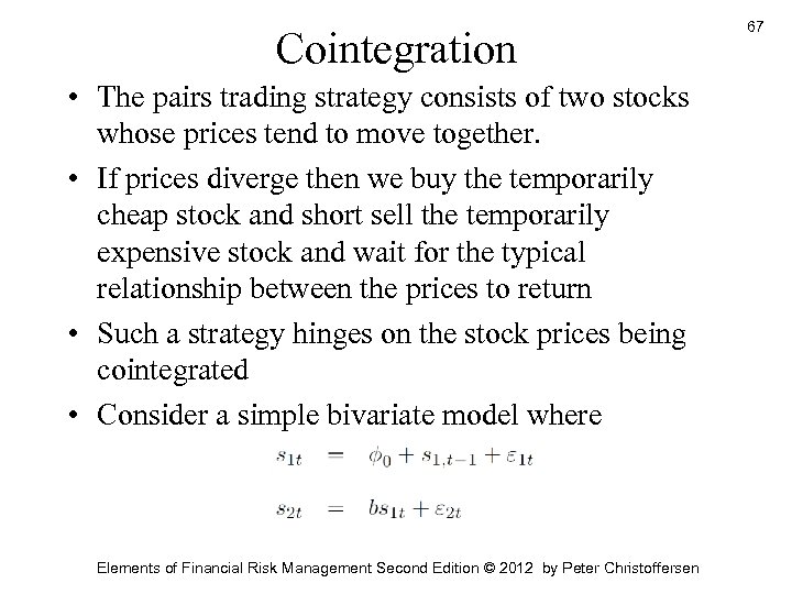Cointegration • The pairs trading strategy consists of two stocks whose prices tend to move together. • If prices diverge then we buy the temporarily cheap stock and short sell the temporarily expensive stock and wait for the typical relationship between the prices to return • Such a strategy hinges on the stock prices being cointegrated • Consider a simple bivariate model where Elements of Financial Risk Management Second Edition © 2012 by Peter Christoffersen 67

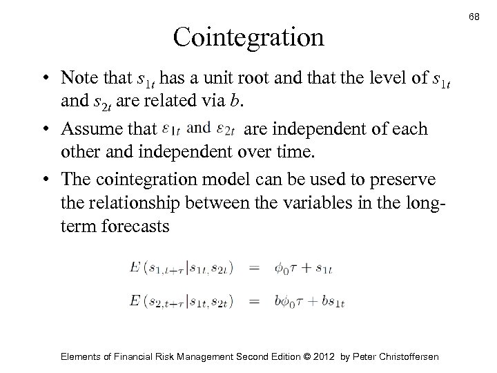Cointegration • Note that s 1 t has a unit root and that the level of s 1 t and s 2 t are related via b. • Assume that are independent of each other and independent over time. • The cointegration model can be used to preserve the relationship between the variables in the longterm forecasts Elements of Financial Risk Management Second Edition © 2012 by Peter Christoffersen 68

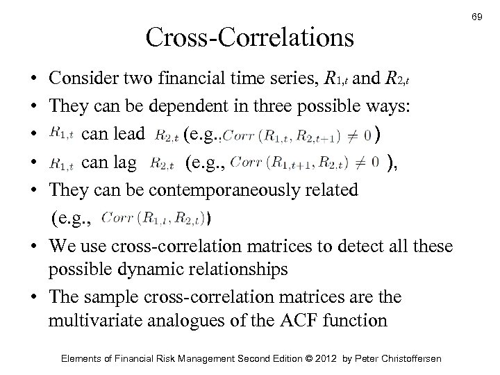Cross-Correlations • Consider two financial time series, R 1, t and R 2, t • They can be dependent in three possible ways: • can lead (e. g. , ) • can lag (e. g. , ), • They can be contemporaneously related (e. g. , ) • We use cross-correlation matrices to detect all these possible dynamic relationships • The sample cross-correlation matrices are the multivariate analogues of the ACF function Elements of Financial Risk Management Second Edition © 2012 by Peter Christoffersen 69

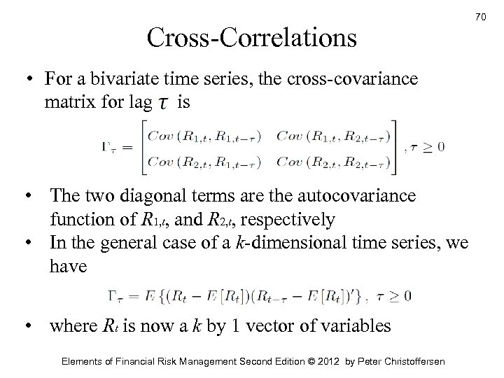Cross-Correlations • For a bivariate time series, the cross-covariance matrix for lag is • The two diagonal terms are the autocovariance function of R 1, t, and R 2, t, respectively • In the general case of a k-dimensional time series, we have • where Rt is now a k by 1 vector of variables Elements of Financial Risk Management Second Edition © 2012 by Peter Christoffersen 70

Cross-Correlations 71 • Detecting lead and lag effects is important • For example, when relating an illiquid stock to a liquid market factor. • The illiquidity of the stock implies price observations that are often stale, which in turn will have a spuriously low correlation with the liquid market factor. • The stale equity price will be correlated with the lagged market factor and this lagged relationship is used to compute a liquidity-corrected measure of the dependence between the stock and the market Elements of Financial Risk Management Second Edition © 2012 by Peter Christoffersen

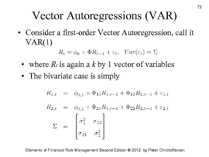Vector Autoregressions (VAR) • Consider a first-order Vector Autoregression, call it VAR(1) • where Rt is again a k by 1 vector of variables • The bivariate case is simply Elements of Financial Risk Management Second Edition © 2012 by Peter Christoffersen 72

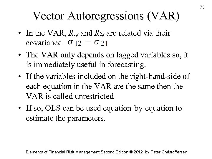Vector Autoregressions (VAR) • In the VAR, R 1, t and R 2, t are related via their covariance • The VAR only depends on lagged variables so, it is immediately useful in forecasting. • If the variables included on the right-hand-side of each equation in the VAR are the same then the VAR is called unrestricted • If so, OLS can be used equation-by-equation to estimate the parameters. Elements of Financial Risk Management Second Edition © 2012 by Peter Christoffersen 73

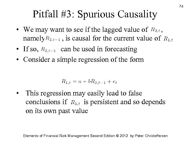Pitfall #3: Spurious Causality • We may want to see if the lagged value of , namely , is causal for the current value of • If so, can be used in forecasting • Consider a simple regression of the form • This regression may easily lead to false conclusions if is persistent and so depends on its own past value Elements of Financial Risk Management Second Edition © 2012 by Peter Christoffersen 74

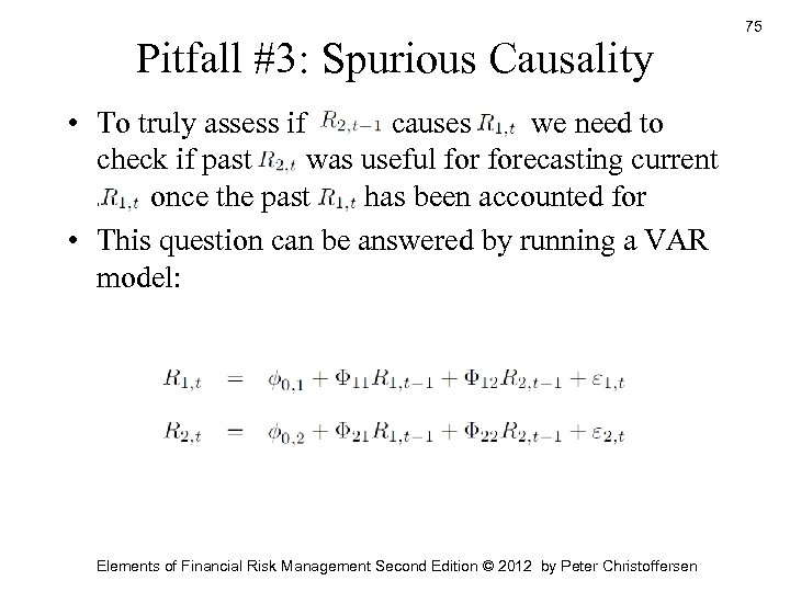Pitfall #3: Spurious Causality • To truly assess if causes we need to check if past was useful forecasting current. once the past has been accounted for • This question can be answered by running a VAR model: Elements of Financial Risk Management Second Edition © 2012 by Peter Christoffersen 75

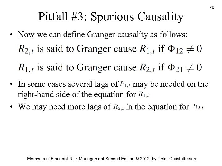Pitfall #3: Spurious Causality • Now we can define Granger causality as follows: • In some cases several lags of may be needed on the right-hand side of the equation for • We may need more lags of in the equation for Elements of Financial Risk Management Second Edition © 2012 by Peter Christoffersen 76

Summary 77 • Financial asset prices and portfolio values can be viewed as examples of very persistent time series • The three most important issues are • Spurious detection of mean reversion-erroneously finding that a variable is mean-reverting when it is truly a random walk • Spurious regression-erroneously finding that a variable x is significant when regressing y on x • Spurious detection of causality-erroneously finding that the current value of x causes future values of y when in reality it cannot Elements of Financial Risk Management Second Edition © 2012 by Peter Christoffersen