03 02 10 Locating and Describing Interest Points Computer Vision

03/02/10 Locating and Describing Interest Points Computer Vision CS 543 / ECE 549 University of Illinois Derek Hoiem Acknowledgment: Many keypoint slides from Grauman&Leibe 2008 AAAI Tutorial

What is “object recognition”?

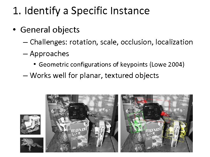
1. Identify a Specific Instance • General objects – Challenges: rotation, scale, occlusion, localization – Approaches • Geometric configurations of keypoints (Lowe 2004) – Works well for planar, textured objects

1. Identify a Specific Instance • Faces – Typical scenario: few examples per face, identify or verify test example – What’s hard: changes in expression, lighting, age, occlusion, viewpoint – Basic approaches (all nearest neighbor) 1. Project into a new subspace (or kernel space) (e. g. , “Eigenfaces”=PCA) 2. Measure face features 3. Make 3 d face model, compare shape+appearance (e. g. , AAM)

2. Detect Instance of a Category • Much harder than specific instance recognition • Challenges – Everything in instance recognition – Intraclass variation – Representation becomes crucial

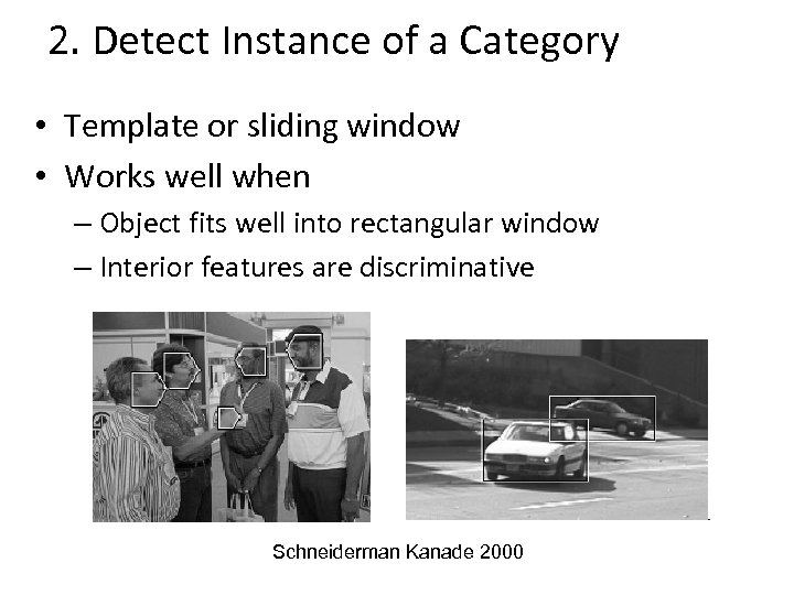
2. Detect Instance of a Category • Template or sliding window • Works well when – Object fits well into rectangular window – Interior features are discriminative Schneiderman Kanade 2000

2. Detect Instance of a Category • Parts-based Fischler and Elschlager 1973 Felzenszwalb et al. 2008

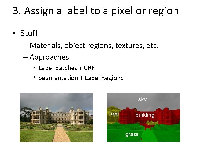
3. Assign a label to a pixel or region • Stuff – Materials, object regions, textures, etc. – Approaches • Label patches + CRF • Segmentation + Label Regions

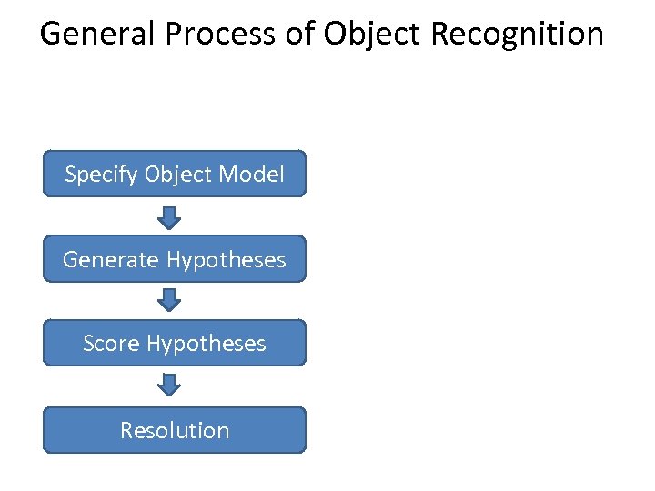
General Process of Object Recognition Specify Object Model Generate Hypotheses Score Hypotheses Resolution

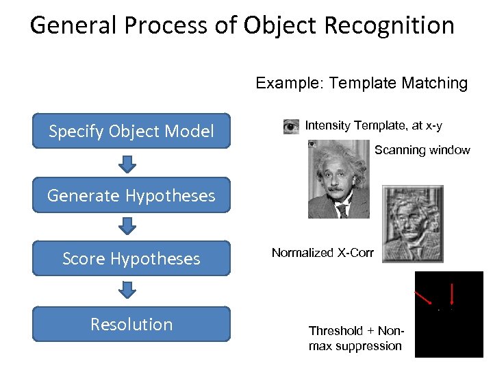
General Process of Object Recognition Example: Template Matching Specify Object Model Intensity Template, at x-y Scanning window Generate Hypotheses Score Hypotheses Resolution Normalized X-Corr Threshold + Nonmax suppression

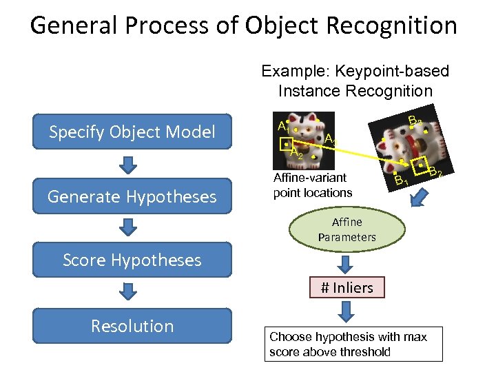
General Process of Object Recognition Example: Keypoint-based Instance Recognition Specify Object Model A 1 A 2 Generate Hypotheses B 3 Affine-variant point locations B 1 Affine Parameters Score Hypotheses # Inliers Resolution Choose hypothesis with max score above threshold B 2

General Process of Object Recognition Example: Keypoint-based Instance Recognition Specify Object Model A 1 A 2 Generate Hypotheses Score Hypotheses Resolution B 3 A 3 B 1 B 2 Today’s Class

Overview of Keypoint Matching 1. Find a set of distinctive keypoints B 3 A 1 A 2 2. Define a region around each keypoint A 3 B 2 B 1 3. Extract and normalize the region content 4. Compute a local descriptor from the normalized region K. Grauman, B. Leibe 5. Match local descriptors

Main challenges • Change in position and scale • Change in viewpoint • Occlusion • Articulation

Goals for Keypoints Detect points that are repeatable and distinctive

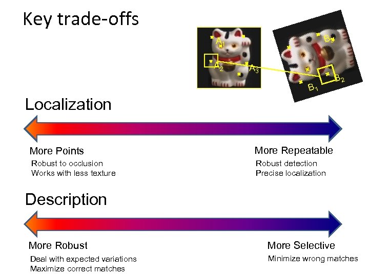
Key trade-offs B 3 A 1 A 2 A 3 B 1 B 2 Localization More Points More Repeatable Robust to occlusion Works with less texture Robust detection Precise localization Description More Robust More Selective Deal with expected variations Maximize correct matches Minimize wrong matches

Keypoint Localization • Goals: – Repeatable detection – Precise localization – Interesting content K. Grauman, B. Leibe

Choosing interest points • If you wanted to meet a friend would you say a) b) c) – “Let’s meet on campus. ” “Let’s meet on Green street. ” “Let’s meet at Green and Wright. ” Corner detection • Or if you were in a secluded area: a) b) c) – “Let’s meet in the Plains of Akbar. ” “Let’s meet on the side of Mt. Doom. ” “Let’s meet on top of Mt. Doom. ” Blob (valley/peak) detection

Choosing interest points • Corners – “Let’s meet at Green and Wright. ” • Peaks/Valleys – “Let’s meet on top of Mt. Doom. ”

Many Existing Detectors Available Hessian & Harris [Beaudet ‘ 78], [Harris ‘ 88] Laplacian, Do. G [Lindeberg ‘ 98], [Lowe 1999] Harris-/Hessian-Laplace [Mikolajczyk & Schmid ‘ 01] Harris-/Hessian-Affine[Mikolajczyk & Schmid ‘ 04] EBR and IBR [Tuytelaars & Van Gool ‘ 04] MSER [Matas ‘ 02] Salient Regions [Kadir & Brady ‘ 01] Others… K. Grauman, B. Leibe

Hessian Detector [Beaudet 78] • Hessian determinant Ixx Iyy Ixy Intuition: Search for strong derivatives in two orthogonal directions K. Grauman, B. Leibe

Hessian Detector [Beaudet 78] • Hessian determinant Ixx Iyy Ixy In Matlab: K. Grauman, B. Leibe

Hessian Detector – Responses [Beaudet 78] Effect: Responses mainly on corners and strongly textured areas.

Hessian Detector – Responses [Beaudet 78]

Harris Detector [Harris 88] • Second moment matrix (autocorrelation matrix) Intuition: Search for local neighborhoods where the image content has two main directions (eigenvectors). K. Grauman, B. Leibe

Harris Detector [Harris 88] • Second moment matrix (autocorrelation matrix) Ix Iy Ix 2 Iy 2 Ix Iy g(Ix 2) g(Iy 2) g(Ix. Iy) 1. Image derivatives 2. Square of derivatives 3. Gaussian filter g(s. I) 4. Cornerness function – both eigenvalues are strong 5. Non-maxima suppression g(Ix. Iy) 32 har

Harris Detector – Responses [Harris 88] Effect: A very precise corner detector.

Harris Detector – Responses [Harris 88]

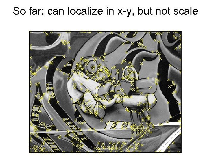
So far: can localize in x-y, but not scale

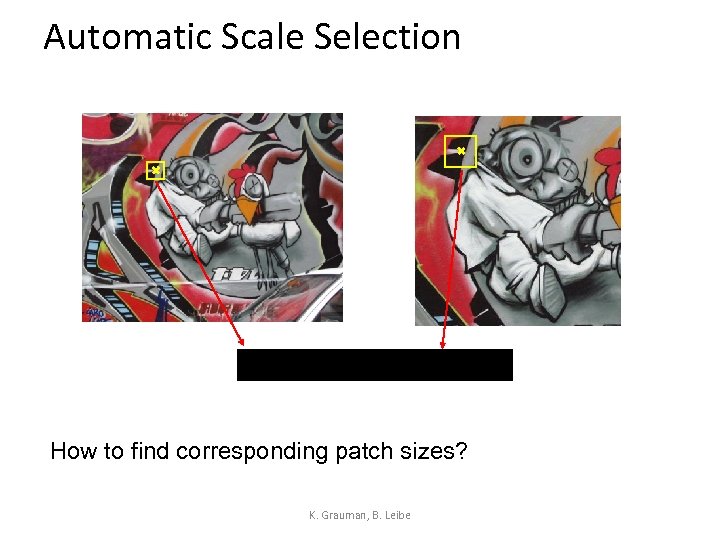
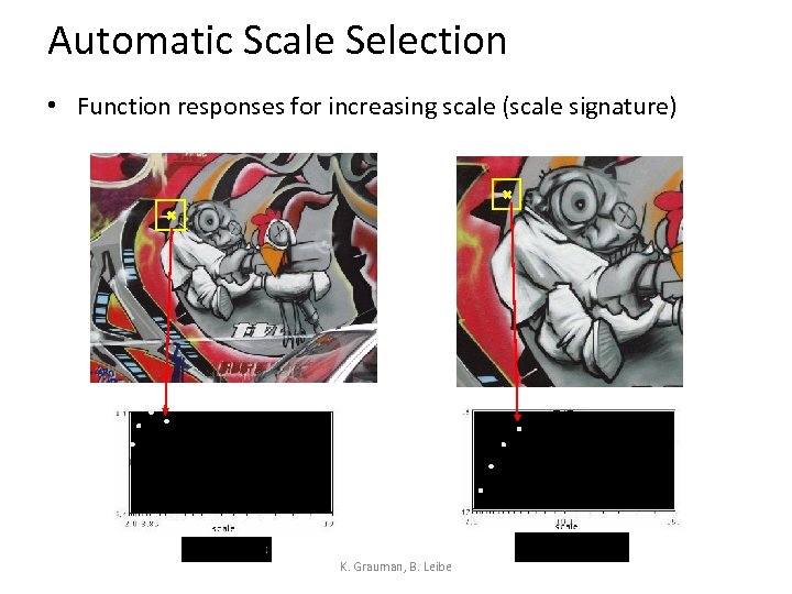
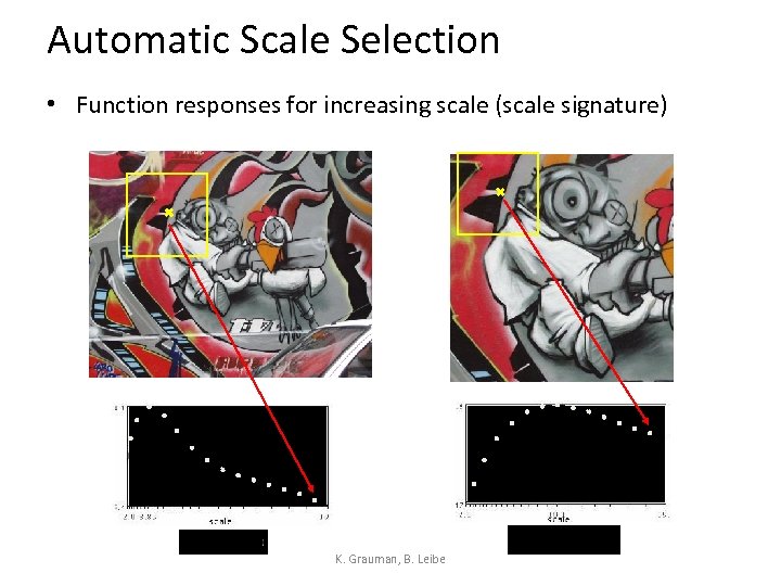
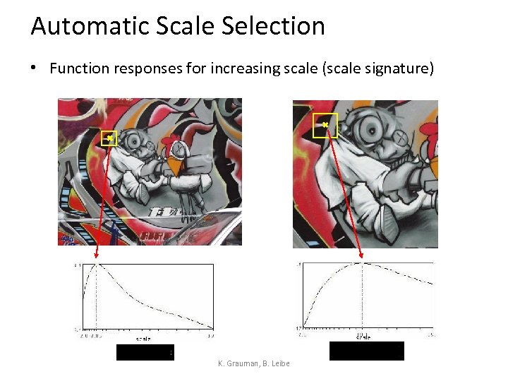
Automatic Scale Selection How to find corresponding patch sizes? K. Grauman, B. Leibe

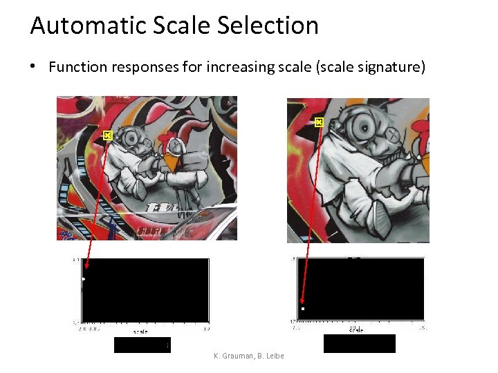
Automatic Scale Selection • Function responses for increasing scale (scale signature) K. Grauman, B. Leibe

Automatic Scale Selection • Function responses for increasing scale (scale signature) K. Grauman, B. Leibe

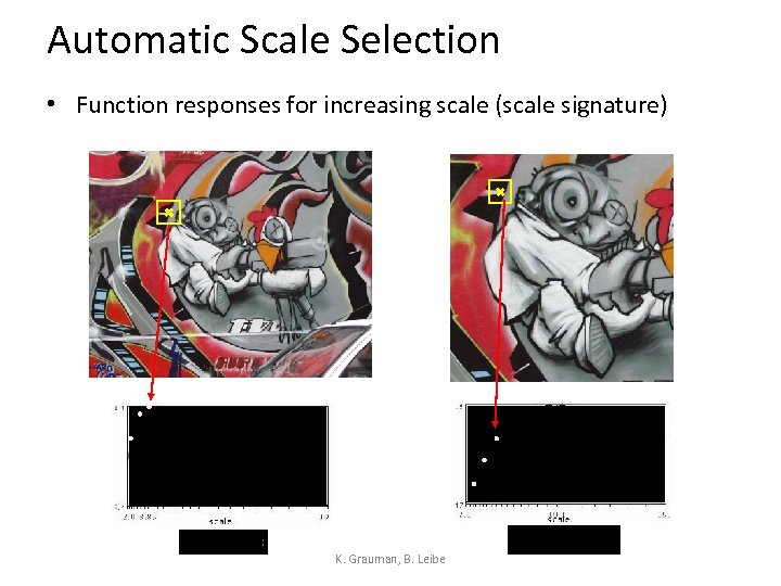
Automatic Scale Selection • Function responses for increasing scale (scale signature) K. Grauman, B. Leibe

Automatic Scale Selection • Function responses for increasing scale (scale signature) K. Grauman, B. Leibe

Automatic Scale Selection • Function responses for increasing scale (scale signature) K. Grauman, B. Leibe

Automatic Scale Selection • Function responses for increasing scale (scale signature) K. Grauman, B. Leibe

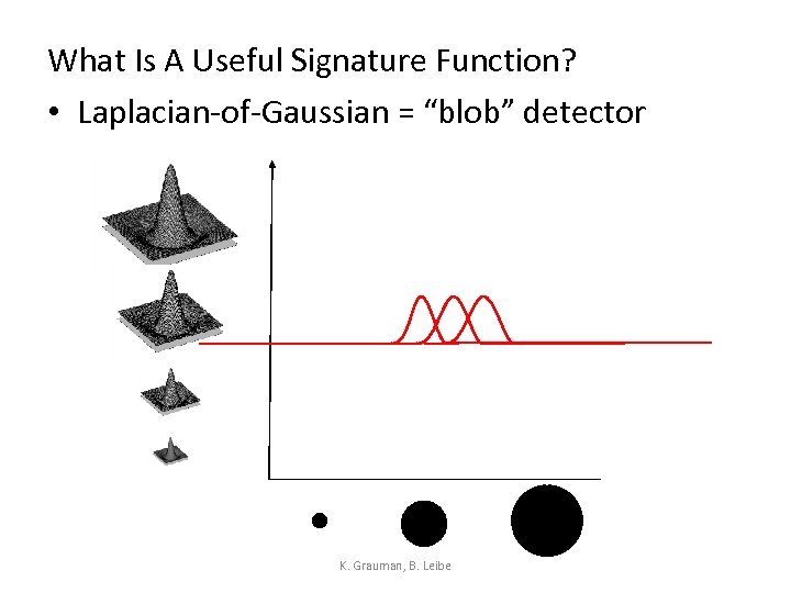
What Is A Useful Signature Function? • Laplacian-of-Gaussian = “blob” detector K. Grauman, B. Leibe

Laplacian-of-Gaussian (Lo. G) • Local maxima in scale space of Laplacian-of-s Gaussian 5 s 4 s 3 s 2 s K. Grauman, B. Leibe List of (x, y, s)

Results: Laplacian-of-Gaussian K. Grauman, B. Leibe

Difference-of-Gaussian (Do. G) • Difference of Gaussians as approximation of the Laplacian-of-Gaussian = - K. Grauman, B. Leibe

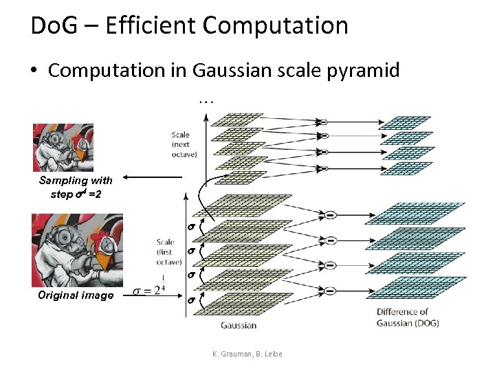
Do. G – Efficient Computation • Computation in Gaussian scale pyramid Sampling with step s 4 =2 s s s Original image s K. Grauman, B. Leibe

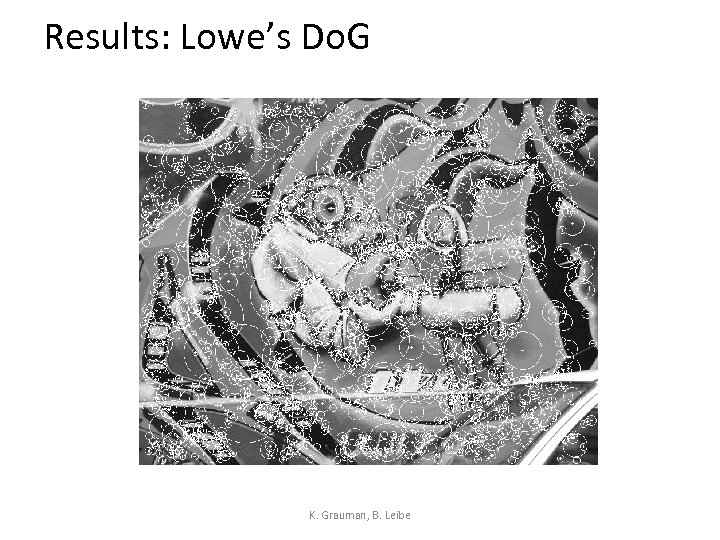
Results: Lowe’s Do. G K. Grauman, B. Leibe

Orientation Normalization • Compute orientation histogram [Lowe, SIFT, 1999] • Select dominant orientation • Normalize: rotate to fixed orientation 0 T. Tuytelaars, B. Leibe 2 p

Harris-Laplace [Mikolajczyk ‘ 01] 1. Initialization: Multiscale Harris corner detection s 4 s 3 s 2 s Computing Harris function Detecting local maxima

Harris-Laplace [Mikolajczyk ‘ 01] 1. Initialization: Multiscale Harris corner detection 2. Scale selection based on Laplacian (same procedure with Hessian-Laplace) Harris points Harris-Laplace points K. Grauman, B. Leibe

Maximally Stable Extremal Regions [Matas ‘ 02] • Based on Watershed segmentation algorithm • Select regions that stay stable over a large parameter range K. Grauman, B. Leibe

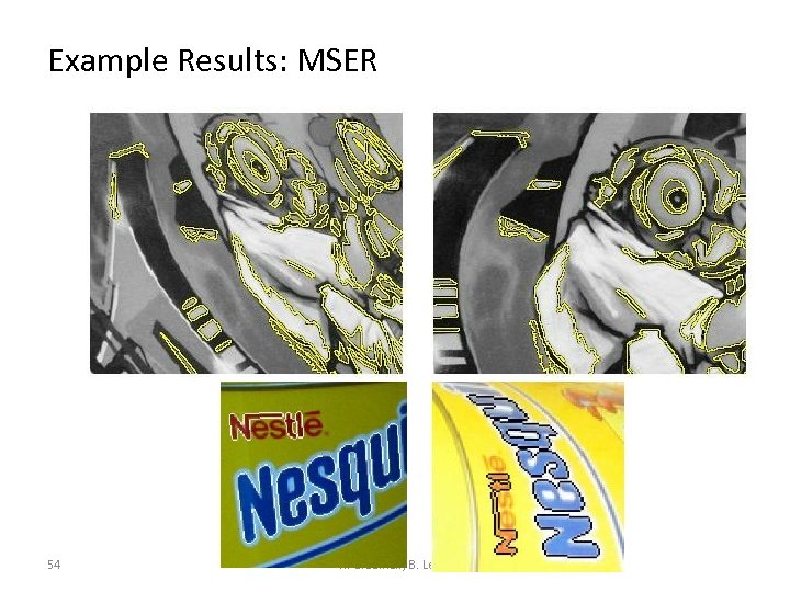
Example Results: MSER 54 K. Grauman, B. Leibe

Available at a web site near you… • For most local feature detectors, executables are available online: – http: //robots. ox. ac. uk/~vgg/research/affine – http: //www. cs. ubc. ca/~lowe/keypoints/ – http: //www. vision. ee. ethz. ch/~surf K. Grauman, B. Leibe

Local Descriptors • The ideal descriptor should be – Robust – Distinctive – Compact – Efficient • Most available descriptors focus on edge/gradient information – Capture texture information – Color rarely used K. Grauman, B. Leibe

Local Descriptors: SIFT Descriptor [Lowe, ICCV 1999] Histogram of oriented gradients • Captures important texture information • Robust to small translations / affine deformations K. Grauman, B. Leibe

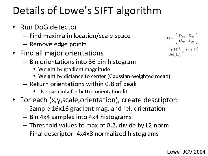
Details of Lowe’s SIFT algorithm • Run Do. G detector – Find maxima in location/scale space – Remove edge points • Find all major orientations – Bin orientations into 36 bin histogram • Weight by gradient magnitude • Weight by distance to center (Gaussian-weighted mean) – Return orientations within 0. 8 of peak • Use parabola for better orientation fit • For each (x, y, scale, orientation), create descriptor: – – Sample 16 x 16 gradient mag. and rel. orientation Bin 4 x 4 samples into 4 x 4 histograms Threshold values to max of 0. 2, divide by L 2 norm Final descriptor: 4 x 4 x 8 normalized histograms Lowe IJCV 2004

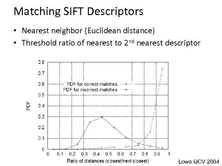
Matching SIFT Descriptors • Nearest neighbor (Euclidean distance) • Threshold ratio of nearest to 2 nd nearest descriptor Lowe IJCV 2004

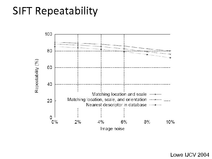
SIFT Repeatability Lowe IJCV 2004

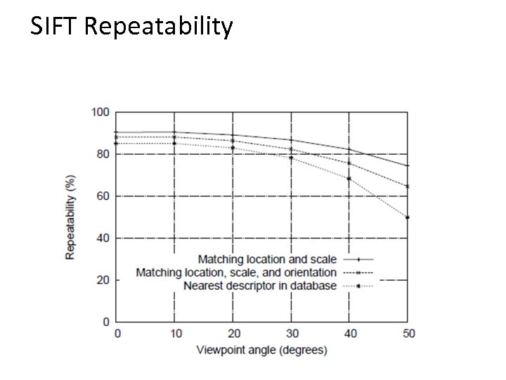
SIFT Repeatability

SIFT Repeatability Lowe IJCV 2004

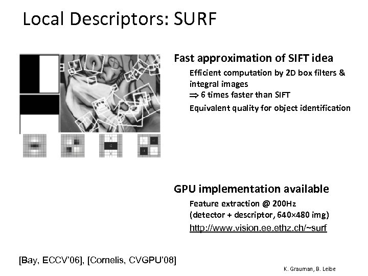
Local Descriptors: SURF • Fast approximation of SIFT idea Ø Ø Efficient computation by 2 D box filters & integral images 6 times faster than SIFT Equivalent quality for object identification • GPU implementation available Ø Ø [Bay, ECCV’ 06], [Cornelis, CVGPU’ 08] Feature extraction @ 200 Hz (detector + descriptor, 640× 480 img) http: //www. vision. ee. ethz. ch/~surf K. Grauman, B. Leibe

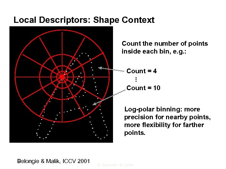
Local Descriptors: Shape Context Count the number of points inside each bin, e. g. : Count = 4. . . Count = 10 Log-polar binning: more precision for nearby points, more flexibility for farther points. Belongie & Malik, ICCV 2001 K. Grauman, B. Leibe

Local Descriptors: Geometric Blur Compute edges at four orientations Extract a patch in each channel ~ Apply spatially varying blur and sub-sample Example descriptor (Idealized signal) Berg & Malik, CVPR 2001 K. Grauman, B. Leibe

Choosing a detector • What do you want it for? – Precise localization in x-y: Harris – Good localization in scale: Difference of Gaussian – Flexible region shape: MSER • Best choice often application dependent – Harris-/Hessian-Laplace/Do. G work well for many natural categories – MSER works well for buildings and printed things • Why choose? – Get more points with more detectors • There have been extensive evaluations/comparisons – [Mikolajczyk et al. , IJCV’ 05, PAMI’ 05] – All detectors/descriptors shown here work well

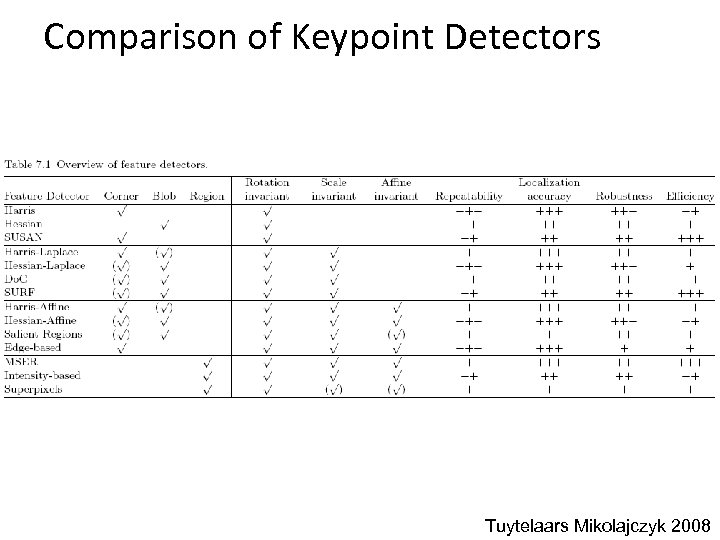
Comparison of Keypoint Detectors Tuytelaars Mikolajczyk 2008

Choosing a descriptor • Again, need not stick to one • For object instance recognition or stitching, SIFT or variant is a good choice

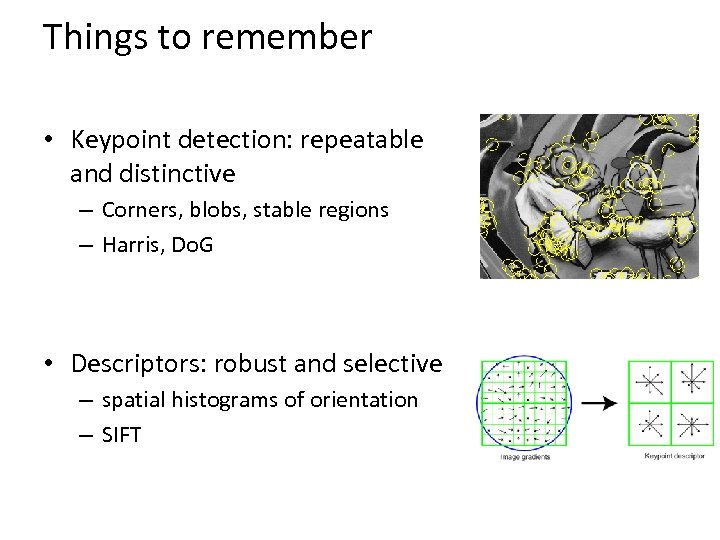
Things to remember • Keypoint detection: repeatable and distinctive – Corners, blobs, stable regions – Harris, Do. G • Descriptors: robust and selective – spatial histograms of orientation – SIFT

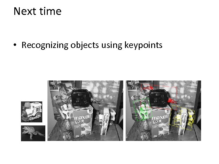
Next time • Recognizing objects using keypoints