Σμήνη Γαλαξιών 28 Ιανουαρίου 2013 Distribution of

Σμήνη Γαλαξιών 28 Ιανουαρίου 2013

Distribution of galaxies Historical remarks • Galaxies are not randomly distributed in space. There are major concentrations of galaxies we refer to as clusters, nearly empty areas that we refer to as voids, and more complicated distributions such as filaments and sheets. • The first written reference to a cluster of galaxies is probably that of Messier in 1784. In his Catalogue, he listed 103 nebulæ, 30 of which we now identify as galaxies. Messier already noticed the exceptional concentration of nebulæ in the Virgo constellation. • Herschel described the Coma cluster (1785) and discovered several clusters (e. g. Hydra) • In 1904 Easton noted an asymmetry in the distribution of the nebulæ with respect to the galactic plane, with an excess of nebulæ in the northern hemisphere (Local Supercluster) • In contrast to the growing dominant opinion, in 1936 Hubble described the distribution of nebulæ as ``moderately uniform'' and noted that ``no organization on a scale larger than the great clusters'' was definitely known. However, he recognized our own Galaxy as a member of a galaxy system, which he named ``The Local Group''. • Zwicky noted that the local group may well be part of the Virgo galaxy system, that Holmberg described as a ``Metagalactic cloud'' of ~ 100 Mpc size. • After the Second World War, the Lick and Palomar sky surveys and the spectroscopic observations of Humason, Mayall & Sandage provided the essential data-base for the analysis of the distribution http: //ned. ipac. caltech. edu/level 5/Biviano 2/paper. pdf of galaxies.

Catalogs of clusters of galaxies • 1957 Herzog, Wild & Zwicky [216] announced the construction of a Catalogue of Galaxies and Clusters of Galaxies [527], that upon completion would contain ~ 10000 clusters. The final CGCG was to be published only in 1967. • Abell's catalogue (1958) The distribution of rich clusters of galaxies, is a milestone in the history of science with galaxy clusters. • Clustering of the nebulæ in the southern and northern hemisphere giving evidence of the Local Supercluster (de Vaucouleurs, 1953) Abell's 2712 clusters were selected on red POSS plates because he realized the advantage of the red band over the blue band for the identification of distant clusters. • Abell's radius was subjectively chosen by looking at the projected overdensities of clusters, and yet is close to the cluster gravitational radius. • Abell, G 1958 Ap. JS. . 3. . 211 A Abell's subjective selection criteria were extremely well chosen, and even the background subtraction was quite accurate. • Abell's paper was much more than a catalogue of clusters. He was the first to show that the distribution of cluster richnesses - which is broadly related to the mass distribution - is very steep.

Optical search for clusters- I: Abell catalog (1958) Abell’s Criteria and his Catalog. • The criteria Abell applied for the identification of clusters refer to an overdensity of galaxies within a specified solid angle. • According to these criteria, a cluster contains ≥ 50 galaxies in a magnitude interval m 3 ≤ m 3+2, where m 3 is the apparent magnitude of the third brightest galaxy in the cluster. • These galaxies must be located within a circle of angular radius θA =1. 7’/z, where z is the estimated redshift. • The latter is determined by the assumption that the luminosity of the tenth brightest galaxy in a cluster is the same for all clusters. • A calibration of this distance estimate is performed on clusters of known redshift. • θA is called the Abell radius of a cluster, and corresponds to a physical radius of RA ≈ 1. 5 h− 1 Mpc. • The so-determined redshift should be within the range 0. 02 ≤ z ≤ 0. 2 for the selection of Abell clusters. • The lower limit is chosen such that a cluster can e found on a single POSS photoplate (6◦Χ 6◦) and does not extend over several plates, which would make the search more difficult, e. g. , because the photographic sensitivity may differ for individual plates. The upper redshift bound is chosen due to the sensitivity limit of the photoplates.

Optical search for clusters- II: Zwicky catalog (19611968) • 18 inch Schmidt gave m. B for 31, 000 galaxies, visual inspection of PSS gave 10, 000 clusters. • Assigned cluster type : Compact, Medium-Compact, Open • Assigned cluster distances : Very Near, Distant, Very Distant, Extremely Distant. • Gave number of galaxies, cluster boundary size, coordinates etc. • Uses "isopleth" density contrast of N / Nbackground = 2 to define cluster, however, statistically incomplete : – cluster sizes are distance dependent • rarely used compared to Abell's lists

Optical search for clusters- III Digitized Surveys Possibly more objective selection criterion uses automated recognition of galaxies and clusters. Main effort : scanning of UK schmidt plates (SRC J & R) by two UK groups : APM (Automatic Plate Measuring Machine) : Cambridge (Mike Irwin et al) COSMOS : Edinburgh/Durham

X-ray Identification of clusters • Rich clusters with deep potentials have hot gas • X-ray emission is an effective way to find relaxed clusters • Since emissivity ~n 2, we have ~ no foreground X-ray emission (though smooth X-ray background) • Problems of spurious identification from superposition is greatly reduced compared to optical surveys. • At high redshifts, this is increasingly important X-ray surveys may be the best way to identify (rich) high-z clusters • • Several surveys currently exist: EMSS (Einstein Medium Sensitivity Survey : serendipitous, 800 deg 2, z 0. 05 - 0. 55) RDCS (ROSAT Deep Cluster Survey : serentipitous, 100 deg 2, z 1) RASS (ROSAT All Sky Survey) XCS (XMM cluster survey) Chandra

The number of X-ray detected clusters is around 5, 000 now with ~500 with measured temperatures and Fe abundances Alastair Edge

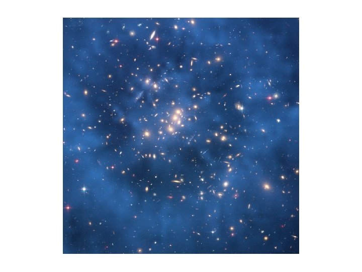
Other Methods of Identification of clusters • SZ (Sunyaev-Zeldovich) effect : Hot cluster gas Compton scatters CMB photons, increasing/decreasing their energy Look for brightening/dimming of CMB at mmwavelengths Promising for detecting high-z clusters Currently very difficult, but recent progress: SPT, PLANCK • Weak Gravitational Lensing : Faint background galaxies suffer slight distortion by matter along the line of sight Intervening clusters give slight azimuthal image elongation Many galaxies statistically detectable Allows mapping of intervening mass distribution. Still early days, but quite promising. • Color Search for Red Galaxies : (Red) Ellipticals formed very early so concentrations of faint red objects should yield high-z clusters Redshift modifies colors, so good color information should also yield approximate redshift.

More on the ZS effect • Scattering of CMB photons by rapidly moving electrons in the hot gas in clusters of galaxies. • These electron-photon collisions redistribute the frequencies of photons in a characteristic way such that, when looking at the CMB in the direction of a galaxy cluster, – one observes a deficit, with respect to the average CMB signal, of low-energy photons, – and a subsequent surplus of more energetic ones. Along the line of sight of a galaxy cluster, the CMB appears fainter at low frequencies and brighter at high frequencies, with the transition value corresponding to 217 GHz. • The signature imprinted by a galaxy cluster on the CMB is thus twofold, consisting of both a negative and a positive signal, and a null effect at 217 GHz. • This characteristic spectral feature enables separation of the SZE from all other anisotropies in the CMB by using observations at several frequencies in the microwave regime. • As a result, the SZE is a unique tool for detecting galaxy clusters, even at high redshift. • The signature of the SZE does not depend on the redshift of the galaxy cluster that produces it

Clusters of galaxies: the bigger picture • Typical cluster sizes are 1 - 3 Mpc : They are the largest virialized structures in the Universe • Structures larger than clusters have not had time to virialize. Galaxies : tvirial ~ 108 yr <<< t. Hubble Clusters : tvirial ~ 109 yr << t. Hubble Superclusters : tvirial ~ 1010. 5 yr > t. Hubble • Note that clusters are not necessarily the largest bound structures in the universe superclusters may be bound, but haven't yet virialized. • Clusters are part of a continuous range of structures : galaxies groups clusters superclusters large scale structure • Clusters are rare extremes in the galaxy distribution, with Δρ/<ρ > ~103 : • Very roughly (depending on definitions) the total galaxy content of the universe is divided : 1 -2% in rich clusters 5 -10% in clusters 50 -100% in "Local Group"s &/or looser groupings

The principal constituents of a cluster The four principal constituents of clusters include: • Galaxies ~102 large galaxies; >103 total galaxies typical speeds ~103 km/s • Intracluster Stars very faint ( 1% sky) diffuse light (distinct from c. D halo light) comprises 10 -50% total galaxy light (in rich clusters; much less in poor clusters) probably tidally stripped stars • Hot Gas Hydrostatic atmosphere T ~107 -8 K X-ray emitter n ~10 -3 cm-3 L~ 1043 -46 erg/s ~ 10 -2 - 10 -4 Lopt Mgas ~ 5 × Mgals Z ~0. 3 Z סּ enriched : not all primordial • Dark Matter Dominates the total mass MDM ~ 4 × Mgas + gals

Clusters of Galaxies – Classification schemes 1) “rich” clusters vs. “poor” clusters Poor clusters include galaxy groups (few to a few dozen members) and clusters with 100’s of members. Masses are 1012 to 1014 solar masses. Rich clusters have 1000’s of members. Masses are 1015 to 1016 solar masses. Higher density of galaxies. 2) “regular” vs. “irregular” clusters Regular clusters have spherical shapes. Tend to be the rich clusters. Irregular clusters have irregular shapes. Tend to be the poor clusters.

Example: Distribution of galaxies (2500 or so) in the Virgo cluster. It is moderately rich but not very regular. Large extension to the south makes it irregular. Also, these galaxies have velocities offset from the main cluster. This is a whole subcluster that is merging with the main cluster.

Characteristics of regular and irregular clusters

The Rood and Sastry classification The Rood and Sastry (RS) classification, is based on the projected distribution classification of the brightest 10 members. They recognize these types: Bautz-Morgan (BM) classifiction: Compares the prominence of the brightest galaxy to the other galaxies. BM I single central dominant c. D galaxy BM II several bright galaxies between c. D and g. E BM III no dominant galaxy

Comparison of the RS and BM classes • The two systems are closely related • it seems there is a primary factor which defines a cluster : its degree of relaxation • from most relaxed to least relaxed we have : BM : I III RS : c. D B L C F I • A number of other properties follow this sequence : Hubble type mix : Elliptical rich Spiral Poor Spiral rich Overall Shape : Spherical Intermediate Irregular X-ray Luminosity : High Intermediate low • It is very likely that this sequence reflects, at least in part, stages in cluster evolution : most evolved intermediate least evolved

The Morphology – Density Relation The higher the density of galaxies, the higher the fraction of ellipticals. Coma cluster: thousands of galaxies, high elliptical fraction

Property/Class Regular Intermediate Irregular Zwicky type Compact Medium-Compact Open Bautz-Morgan type I, I-II, II (II), II-III (II-III), III Rood-Sastry type c. D, B, (L, C) (L), (F), (C) (F), I Content Elliptical-rich Spiral-poor Spiral-rich E: S 0: S ratio 3: 4: 2 1: 2: 3 Symmetry Spherical Intermediate Irregular shape Central concentration High Moderate Very little Central profile Steep Intermediate Flat Mass segregation ? Marginal None Radio detection ? 50% 20% X-ray luminosity High Intermediate Low Examples A 2199, Coma A 194, A 539 Virgo, A 1228

Important Timescales

Cluster Shapes & Kinematics

Cluster Shapes & Kinematics-contnd • Analytically : Following violent relaxation, we expect : isothermal and isotropic velocity distribution an equilibrium stellar dynamical system of this kind has (r) with : flat core, core radius, & steep r-2 envelope appropriate solutions include : isothermal profile or King profile or analytic equivalents eg ρ(r) = ρ(0) [1 + (r/rc)2]-3/2 • Numerically : Collisionless collapse simulations suggest a profile more similar to Σ(R)~R 1/4 de Vaucouleurs law (not surprisingly, since the calculation is similar to collapse/merger in elliptical formation) Observed profiles fit both this and the analytic profiles equally well. Substructures

Large-scale structures • Superclusters: These usually consist of chains of about a dozen clusters which have a mass of about 10^16 solar masses (ten million billion suns). Our own Local Supercluster is centred on Virgo and is relatively poor having a size of 15 Mpc. The largest superclusters, like that associated with Coma, are up to 100 Mpc in extent. The system of superclusters forms a network permeating throughout space, on which about 90% of galaxies are located. • The Great Attractor: Measurements of peculiar velocities---deviations away from the Hubble flow - are achieved by comparing redshifts and galactic distance indicators. These have revealed enormous coherent motions on scales in excess of 60 Mpc. Consistent with these flows, our own galaxy is moving at about 600 km/s towards a distant object dubbed the `Great Attractor'. This lies at a distance of 45 Mpc and has a mass approaching 5 x 10^16 solar masses. • Voids, sheets & filaments: Deep redshift surveys reveal a very bubbly structure to the universe with galaxies primarily confined to sheets and filaments. Voids are the dominant feature and have a typical diameter of about 25 Mpc. They fill about 90% of space and the largest observed, Bootes void, has a diameter of about 124 Mpc. Other features that have been observed are the `Great Wall', an apparent sheet of galaxies 100 Mpc long at a distance of about 100 Mpc.

Two-point correlation function • The two-point correlation function is one of the main statistics used for description of the galaxy distribution. • The standard statistical analysis assumes that the objects can be regarded as point particles and these particles are assumed to be distributed homogeneously on a suﬃciently large scale within the sample boundaries. • This means that we can meaningfully assign an average number density to the distribution. • Therefore, we can characterize the galaxy distribution in terms of the extent of the departures from uniformity on various scales. • According to Peebles the two-point correlation function ξ(r) determines a probability d. P to find simultaneously two objects on a distance r from each other within two volume elements δV 1 and δV 2 in a sample with number density n as • d. P=n 2[1+ξ(r)]δV 1δV 2. • This correlation function (when one speaks about a distribution of objects of one type) is also known as autocorrelation function.

The Local (Virgo)Supercluster Assemblages of clusters and groups

More Superclusters – note the filamentary shapes

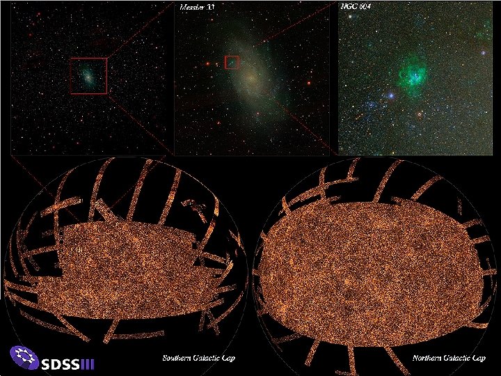
• Total area on sky ~ 2000 deg 2 • 250, 000 galaxies in total, 93% sampling rate • Mean redshift <z> ~ 0. 1, almost all with z < 0. 3

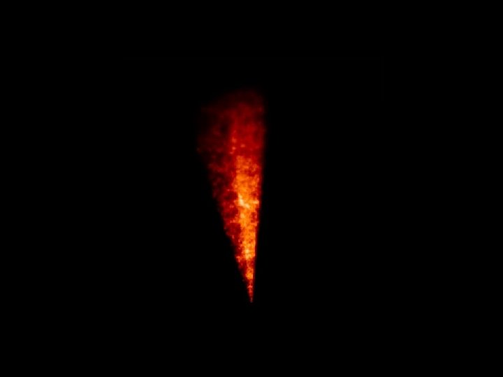
3 D-slice Galaxy Map SDSS

2 d. F galaxy Redshift survey