Statistika Chapter 12 Simple Regression Introduction to

Statistika Chapter 12 Simple Regression

Introduction to Regression Analysis Analisis regresi adalah analisis hubungan linear antar 2 variabel random yang mempunyai hub linear, Variabel bebas (variabel pengaruh) Variabel respon (variabel terpengaruh) Regression analysis is used to: Predict the value of a dependent variable (Y) based on the value of at least one independent variable (X) Explain the impact of changes in an independent variable on the dependent variable Dependent variable: the variable we wish to explain Independent variable: the variable used to explain the dependent variable

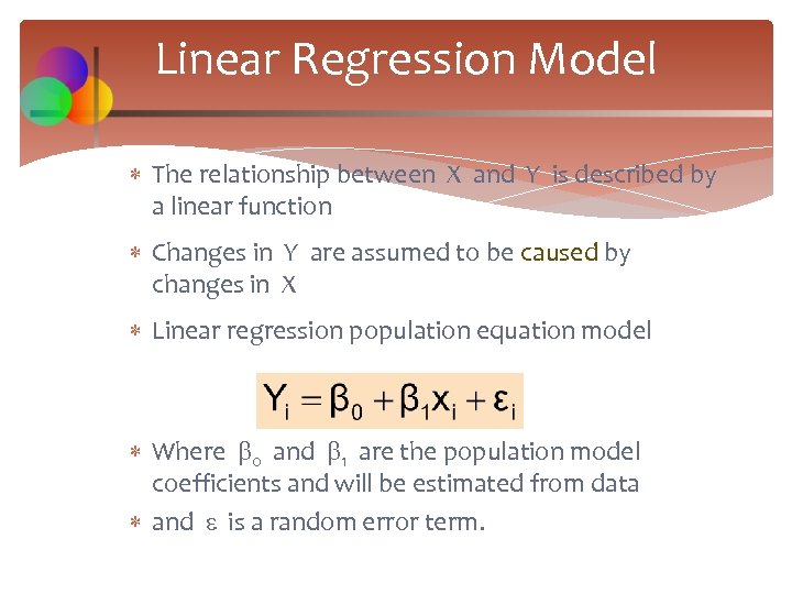Linear Regression Model The relationship between X and Y is described by a linear function Changes in Y are assumed to be caused by changes in X Linear regression population equation model Where 0 and 1 are the population model coefficients and will be estimated from data and is a random error term.

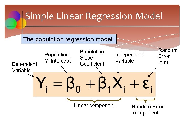Simple Linear Regression Model The population regression model: Dependent Variable Population Y intercept Population Slope Coefficient Linear component Independent Variable Random Error term Random Error component

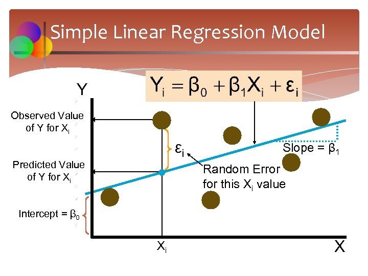Simple Linear Regression Model Y Observed Value of Y for Xi εi Predicted Value of Y for Xi Slope = β 1 Random Error for this Xi value Intercept = β 0 Xi X

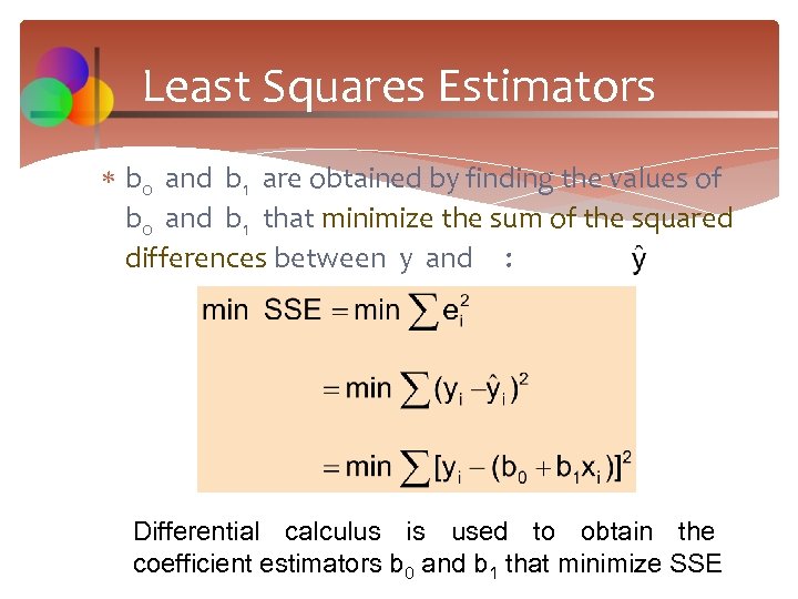Least Squares Estimators b 0 and b 1 are obtained by finding the values of b 0 and b 1 that minimize the sum of the squared differences between y and : Differential calculus is used to obtain the coefficient estimators b 0 and b 1 that minimize SSE

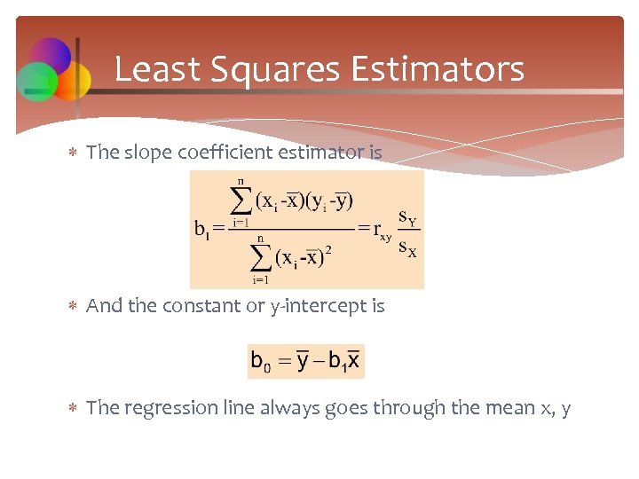Least Squares Estimators The slope coefficient estimator is And the constant or y-intercept is The regression line always goes through the mean x, y

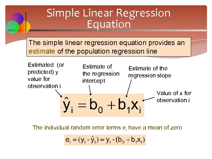Simple Linear Regression Equation The simple linear regression equation provides an estimate of the population regression line Estimated (or predicted) y value for observation i Estimate of the regression intercept Estimate of the regression slope Value of x for observation i The individual random error terms ei have a mean of zero

Finding the Least Squares Equation The coefficients b 0 and b 1 , and other regression results in this chapter, will be found using a computer Hand calculations are tedious (boring) Statistical routines are built into Excel Other statistical analysis software can be used

Interpretation of the Slope and the Intercept b 0 is the estimated average value of y when the value of x is zero (if x = 0 is in the range of observed x values) b 1 is the estimated change in the average value of y as a result of a one-unit change in x

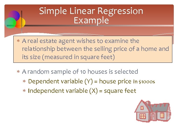Simple Linear Regression Example A real estate agent wishes to examine the relationship between the selling price of a home and its size (measured in square feet) A random sample of 10 houses is selected Dependent variable (Y) = house price in $1000 s Independent variable (X) = square feet

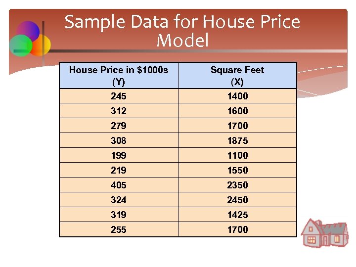Sample Data for House Price Model House Price in $1000 s (Y) Square Feet (X) 245 1400 312 1600 279 1700 308 1875 199 1100 219 1550 405 2350 324 2450 319 1425 255 1700

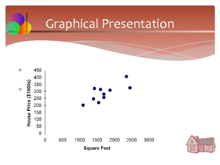Graphical Presentation House price model: scatter plot From the scatter plot there is a linear trend

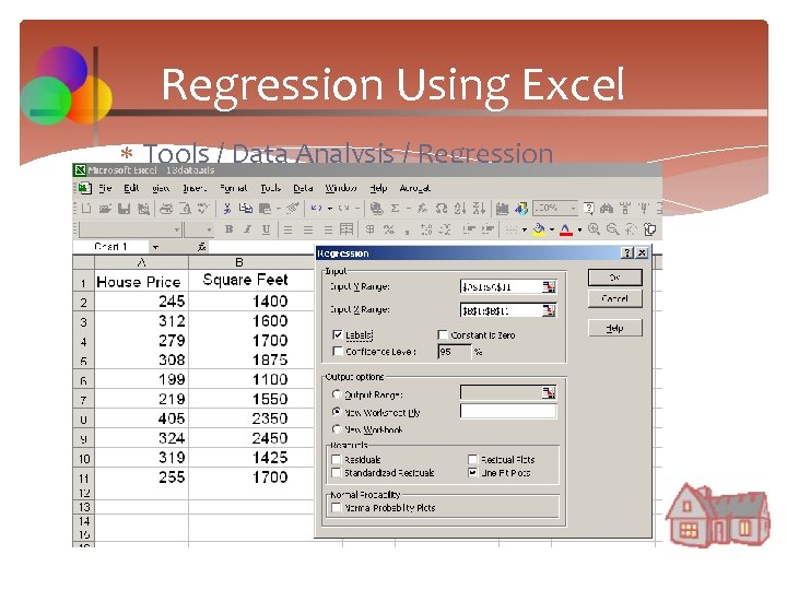Regression Using Excel Tools / Data Analysis / Regression

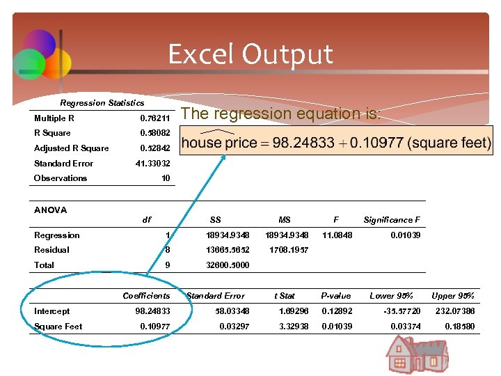Excel Output Regression Statistics Multiple R 0. 76211 R Square 0. 58082 Adjusted R Square The regression equation is: 0. 52842 Standard Error 41. 33032 Observations 10 ANOVA df SS MS Regression 1 18934. 9348 Residual 8 13665. 5652 9 32600. 5000 Significance F 1708. 1957 Total F Intercept Square Feet Coefficients Standard Error 11. 0848 t Stat 0. 01039 P-value Lower 95% Upper 95% 98. 24833 58. 03348 1. 69296 0. 12892 -35. 57720 232. 07386 0. 10977 0. 03297 3. 32938 0. 01039 0. 03374 0. 18580

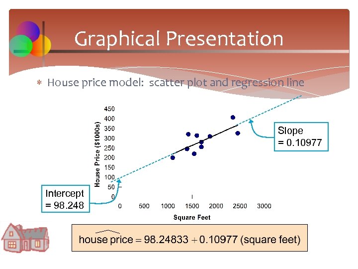Graphical Presentation House price model: scatter plot and regression line Slope = 0. 10977 Intercept = 98. 248

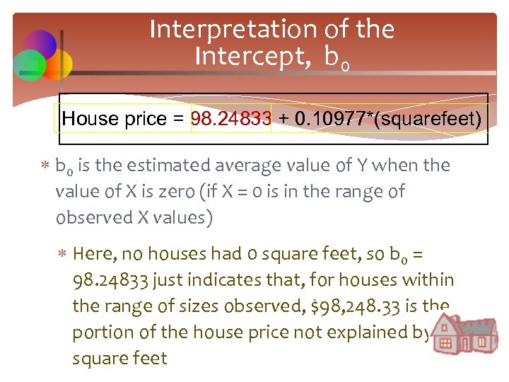Interpretation of the Intercept, b 0 House price = 98. 24833 + 0. 10977*(squarefeet) b 0 is the estimated average value of Y when the value of X is zero (if X = 0 is in the range of observed X values) Here, no houses had 0 square feet, so b 0 = 98. 24833 just indicates that, for houses within the range of sizes observed, $98, 248. 33 is the portion of the house price not explained by square feet

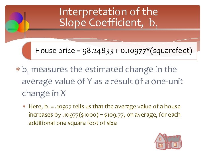Interpretation of the Slope Coefficient, b 1 House price = 98. 24833 + 0. 10977*(squarefeet) b 1 measures the estimated change in the average value of Y as a result of a one-unit change in X Here, b 1 =. 10977 tells us that the average value of a house increases by. 10977($1000) = $109. 77, on average, for each additional one square foot of size