STAT6202 Chapter 1 2012/2013 1 STAT6202: Introductory Statistical

STAT6202 Chapter 1 2012/2013 1 STAT6202: Introductory Statistical Methods (B) Dr. Vera Raats Email: [email protected] Office hours: ? Office: Room 140, 1-19 Torrington Place Course website: Moodle

STAT6202 Chapter 1 2012/2013 2 ADMINISTRATION COURSE SET-UP Weekly lectures: 2 hours Weekly compulsory tutorials: 1 hour COURSE NOTES AND BOOKS Print a copy of the course notes yourself Supplementary reading list (not compulsory) COURSE ASSESSMENT Two parts ICA (20%): 45 minutes on 14Nov2012 Exam (80%): 2.5 hours in term 3 Both open book (any printed/written material) and compulsory CALCULATORS: only college approved ones are allowed MOODLE COURSE WEBSITE: enrolment key is Milly6202

STAT6202 Chapter 1 2012/2013 3 CHAPTER 1 Data summary and presentation POPULATION AND SAMPLES TYPES OF VARIABLES SUMMARY STATISTICS TABLES AND GRAPHS BOXPLOT AND SKEWNESS LINEAR TRANSFORMATIONS LOG TRANSFORMATIONS

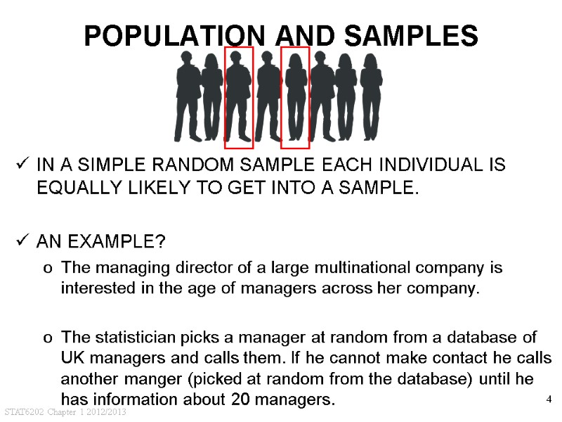
STAT6202 Chapter 1 2012/2013 4 POPULATION AND SAMPLES IN A SIMPLE RANDOM SAMPLE EACH INDIVIDUAL IS EQUALLY LIKELY TO GET INTO A SAMPLE. AN EXAMPLE? The managing director of a large multinational company is interested in the age of managers across her company. The statistician picks a manager at random from a database of UK managers and calls them. If he cannot make contact he calls another manger (picked at random from the database) until he has information about 20 managers.

STAT6202 Chapter 1 2012/2013 5 POPULATION AND SAMPLES Drawing a simple random sample ASSIGN A UNIQUE NUMBER TO EACH MEMBER OF POPULATION. THEN DRAW RANDOM NUMBERS. One option: Table 1 Another (often used) option: Computer randomly generated numbers SAMPLE CONSISTS OF POPULATION MEMBERS WITH (RANDOMLY) SELECTED NUMBERS.

STAT6202 Chapter 1 2012/2013 6 CHAPTER 1 Data summary and presentation POPULATION AND SAMPLES TYPES OF VARIABLES SUMMARY STATISTICS TABLES AND GRAPHS BOXPLOT AND SKEWNESS LINEAR TRANSFORMATIONS LOG TRANSFORMATIONS

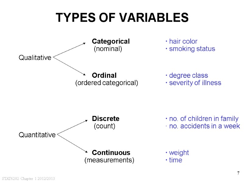
STAT6202 Chapter 1 2012/2013 7 TYPES OF VARIABLES Categorical · hair color (nominal) · smoking status Qualitative Ordinal · degree class (ordered categorical) · severity of illness Discrete · no. of children in family (count) · no. accidents in a week Quantitative Continuous · weight (measurements) · time

STAT6202 Chapter 1 2012/2013 8 CHAPTER 1 Data summary and presentation POPULATION AND SAMPLES TYPES OF VARIABLES SUMMARY STATISTICS TABLES AND GRAPHS BOXPLOT AND SKEWNESS LINEAR TRANSFORMATIONS LOG TRANSFORMATIONS

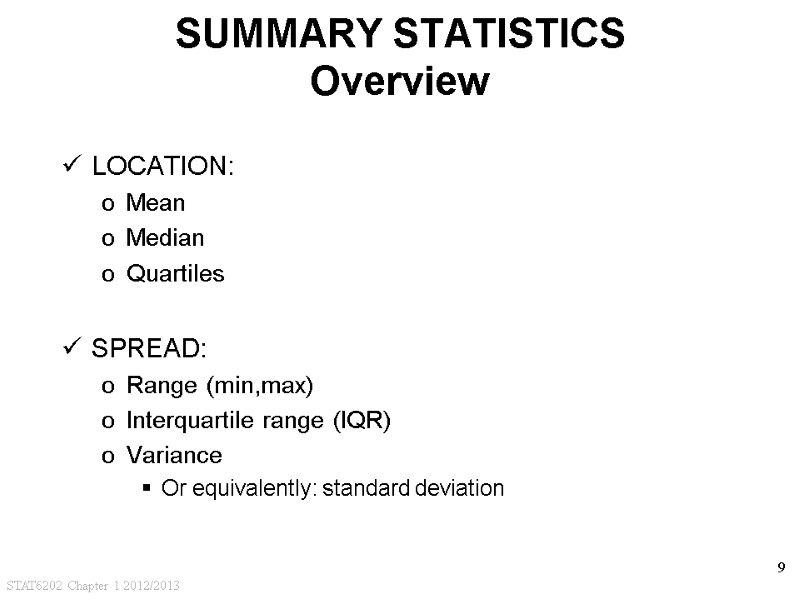
STAT6202 Chapter 1 2012/2013 9 SUMMARY STATISTICS Overview LOCATION: Mean Median Quartiles SPREAD: Range (min,max) Interquartile range (IQR) Variance Or equivalently: standard deviation

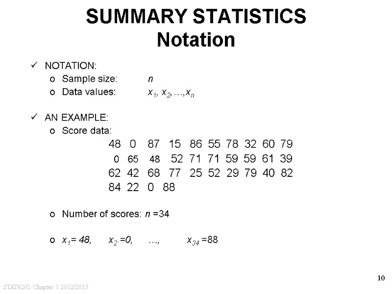
STAT6202 Chapter 1 2012/2013 10 SUMMARY STATISTICS Notation NOTATION: Sample size: n Data values: x1, x2,…,xn AN EXAMPLE: Score data: 48 0 87 15 86 55 78 32 60 79 0 65 48 52 71 71 59 59 61 39 62 42 68 77 25 52 29 79 40 82 84 22 0 88 Number of scores: n =34 x1= 48, x2 =0, …, x34 =88

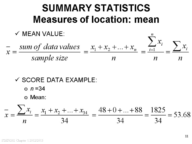
STAT6202 Chapter 1 2012/2013 11 SUMMARY STATISTICS Measures of location: mean MEAN VALUE: SCORE DATA EXAMPLE: n =34 Mean:

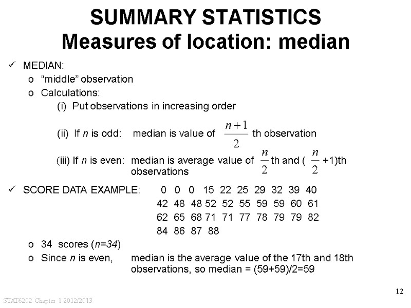
STAT6202 Chapter 1 2012/2013 12 SUMMARY STATISTICS Measures of location: median MEDIAN: “middle” observation Calculations: (i) Put observations in increasing order (ii) If n is odd: median is value of th observation (iii) If n is even: median is average value of th and ( +1)th observations SCORE DATA EXAMPLE: 0 0 0 15 22 25 29 32 39 40 42 48 48 52 52 55 59 59 60 61 62 65 68 71 71 77 78 79 79 82 84 86 87 88 34 scores (n=34) Since n is even, median is the average value of the 17th and 18th observations, so median = (59+59)/2=59

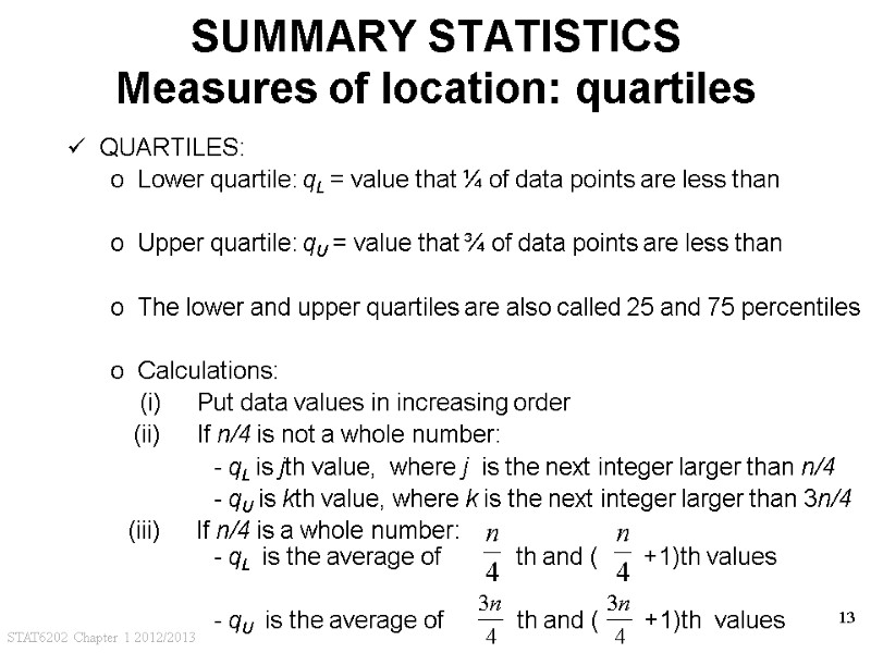
STAT6202 Chapter 1 2012/2013 13 SUMMARY STATISTICS Measures of location: quartiles QUARTILES: Lower quartile: qL = value that ¼ of data points are less than Upper quartile: qU = value that ¾ of data points are less than The lower and upper quartiles are also called 25 and 75 percentiles Calculations: (i) Put data values in increasing order (ii) If n/4 is not a whole number: - qL is jth value, where j is the next integer larger than n/4 - qU is kth value, where k is the next integer larger than 3n/4 (iii) If n/4 is a whole number: - qL is the average of th and ( +1)th values - qU is the average of th and ( +1)th values

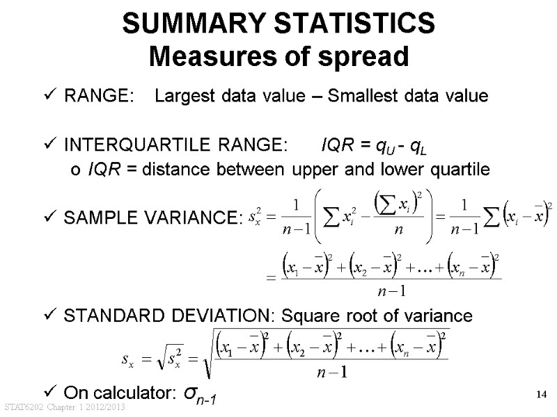
STAT6202 Chapter 1 2012/2013 14 SUMMARY STATISTICS Measures of spread RANGE: Largest data value – Smallest data value INTERQUARTILE RANGE: IQR = qU - qL IQR = distance between upper and lower quartile SAMPLE VARIANCE: STANDARD DEVIATION: Square root of variance On calculator: σn-1

STAT6202 Chapter 1 2012/2013 15 CHAPTER 1 Data summary and presentation POPULATION AND SAMPLES TYPES OF VARIABLES SUMMARY STATISTICS TABLES AND GRAPHS BOXPLOT AND SKEWNESS LINEAR TRANSFORMATIONS LOG TRANSFORMATIONS

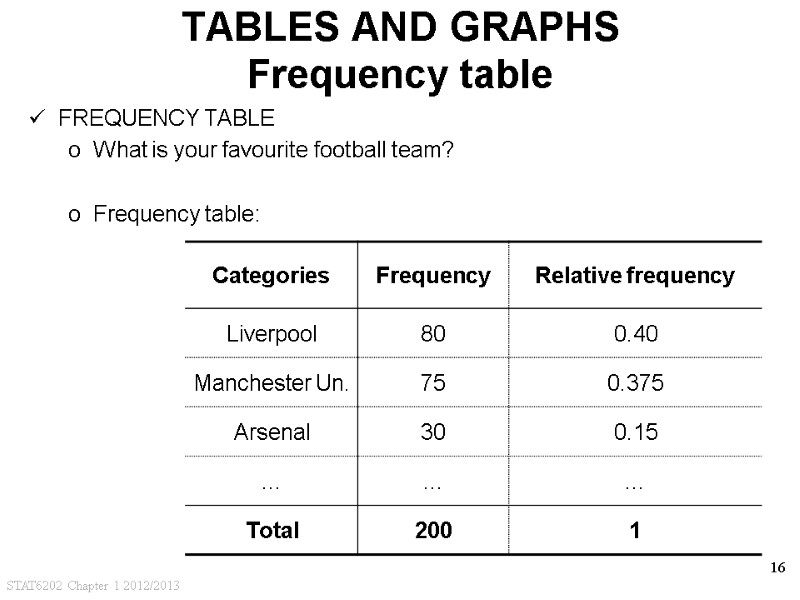
STAT6202 Chapter 1 2012/2013 16 TABLES AND GRAPHS Frequency table FREQUENCY TABLE What is your favourite football team? Frequency table:

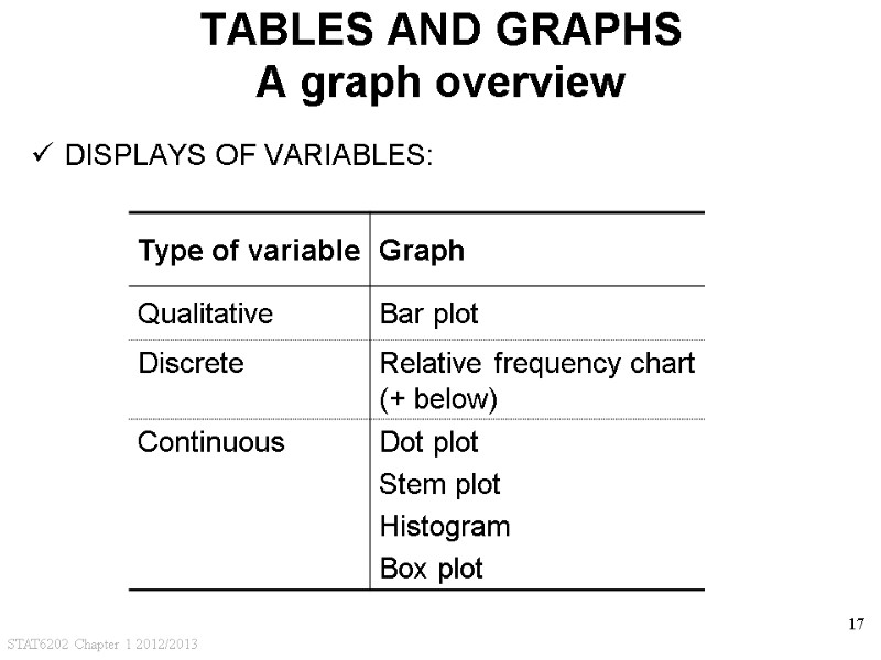
STAT6202 Chapter 1 2012/2013 17 TABLES AND GRAPHS A graph overview DISPLAYS OF VARIABLES:

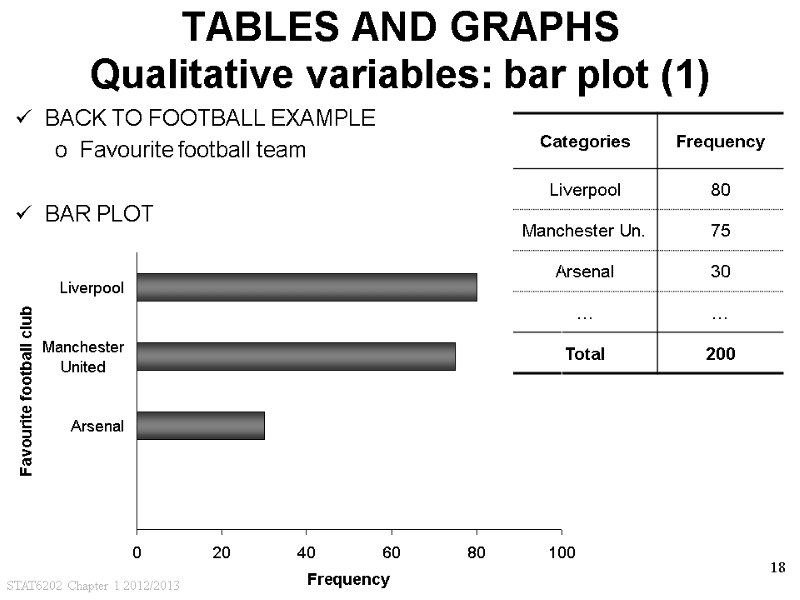
STAT6202 Chapter 1 2012/2013 18 TABLES AND GRAPHS Qualitative variables: bar plot (1) BACK TO FOOTBALL EXAMPLE Favourite football team BAR PLOT

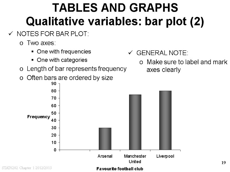
STAT6202 Chapter 1 2012/2013 19 TABLES AND GRAPHS Qualitative variables: bar plot (2) NOTES FOR BAR PLOT: Two axes: One with frequencies One with categories Length of bar represents frequency Often bars are ordered by size GENERAL NOTE: Make sure to label and mark axes clearly

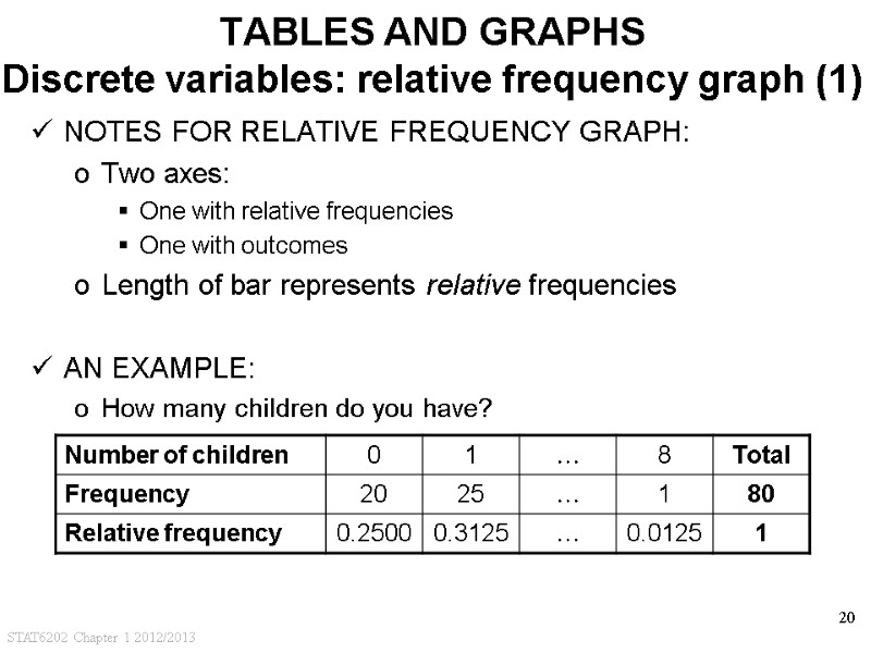
STAT6202 Chapter 1 2012/2013 20 TABLES AND GRAPHS Discrete variables: relative frequency graph (1) NOTES FOR RELATIVE FREQUENCY GRAPH: Two axes: One with relative frequencies One with outcomes Length of bar represents relative frequencies AN EXAMPLE: How many children do you have?

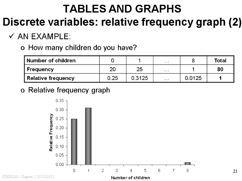
STAT6202 Chapter 1 2012/2013 21 TABLES AND GRAPHS Discrete variables: relative frequency graph (2) AN EXAMPLE: How many children do you have? Relative frequency graph

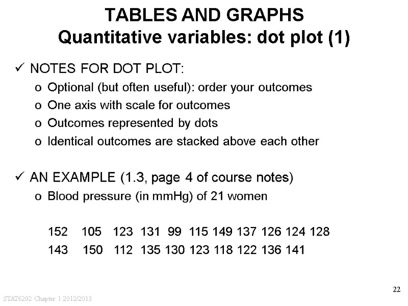
STAT6202 Chapter 1 2012/2013 22 TABLES AND GRAPHS Quantitative variables: dot plot (1) NOTES FOR DOT PLOT: Optional (but often useful): order your outcomes One axis with scale for outcomes Outcomes represented by dots Identical outcomes are stacked above each other AN EXAMPLE (1.3, page 4 of course notes) Blood pressure (in mmHg) of 21 women 152 105 123 131 99 115 149 137 126 124 128 143 150 112 135 130 123 118 122 136 141

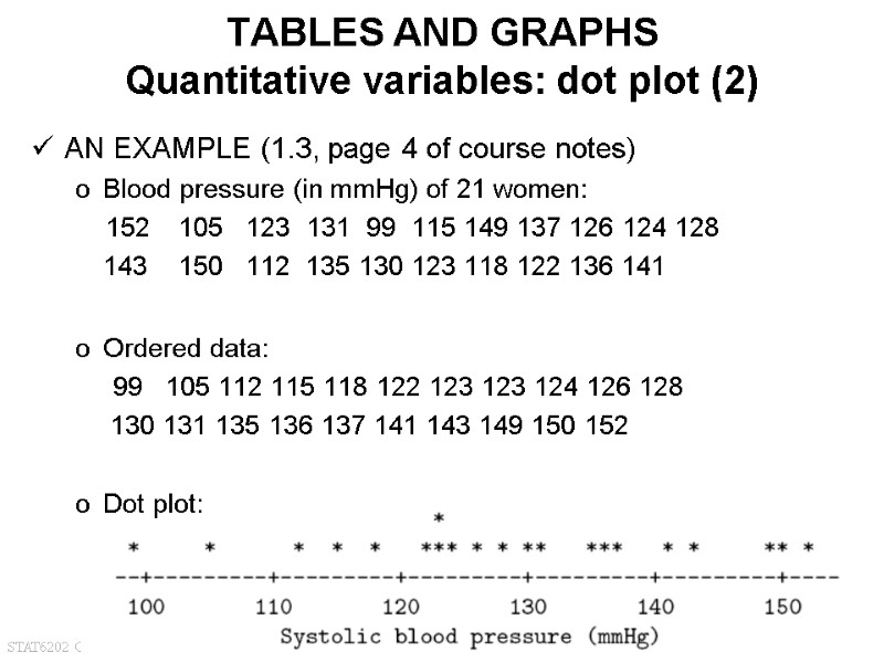
STAT6202 Chapter 1 2012/2013 23 TABLES AND GRAPHS Quantitative variables: dot plot (2) AN EXAMPLE (1.3, page 4 of course notes) Blood pressure (in mmHg) of 21 women: 152 105 123 131 99 115 149 137 126 124 128 143 150 112 135 130 123 118 122 136 141 Ordered data: 99 105 112 115 118 122 123 123 124 126 128 130 131 135 136 137 141 143 149 150 152 Dot plot:

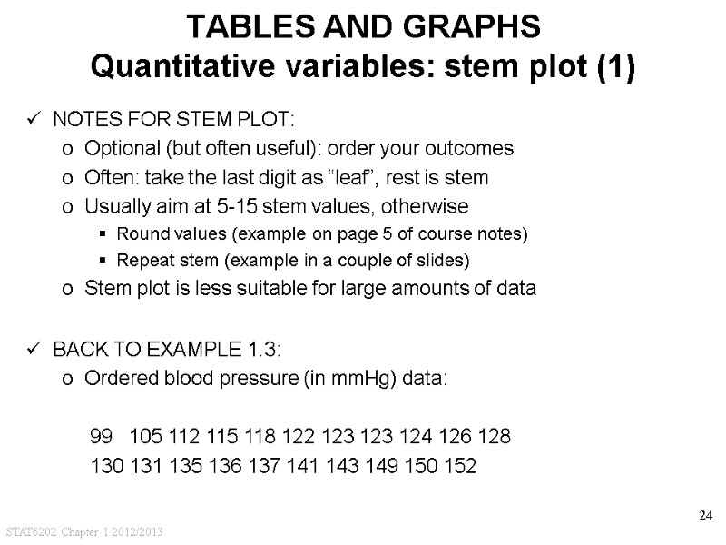
STAT6202 Chapter 1 2012/2013 24 TABLES AND GRAPHS Quantitative variables: stem plot (1) NOTES FOR STEM PLOT: Optional (but often useful): order your outcomes Often: take the last digit as “leaf”, rest is stem Usually aim at 5-15 stem values, otherwise Round values (example on page 5 of course notes) Repeat stem (example in a couple of slides) Stem plot is less suitable for large amounts of data BACK TO EXAMPLE 1.3: Ordered blood pressure (in mmHg) data: 99 105 112 115 118 122 123 123 124 126 128 130 131 135 136 137 141 143 149 150 152

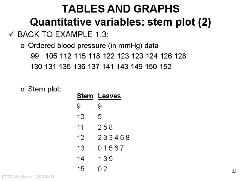
STAT6202 Chapter 1 2012/2013 25 TABLES AND GRAPHS Quantitative variables: stem plot (2) BACK TO EXAMPLE 1.3: Ordered blood pressure (in mmHg) data 99 105 112 115 118 122 123 123 124 126 128 130 131 135 136 137 141 143 149 150 152 Stem plot:

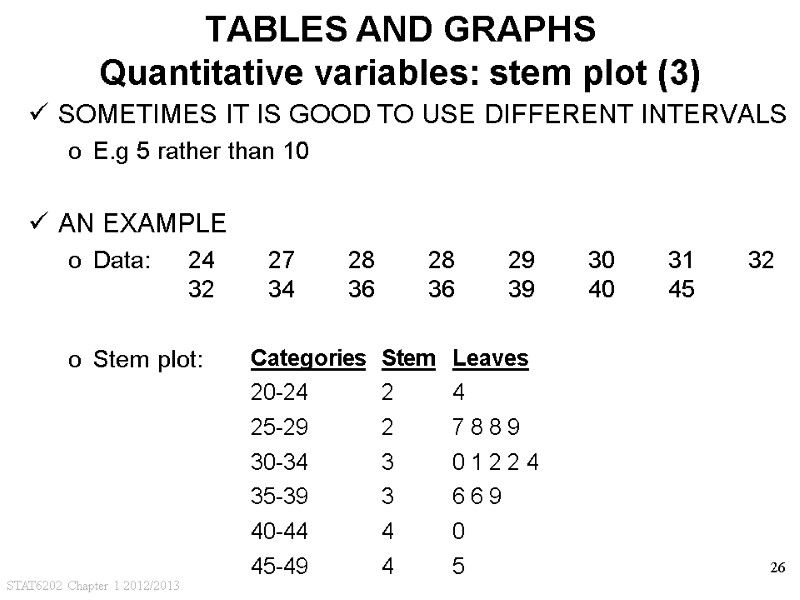
STAT6202 Chapter 1 2012/2013 26 TABLES AND GRAPHS Quantitative variables: stem plot (3) SOMETIMES IT IS GOOD TO USE DIFFERENT INTERVALS E.g 5 rather than 10 AN EXAMPLE Data: 24 27 28 28 29 30 31 32 32 34 36 36 39 40 45 Stem plot:

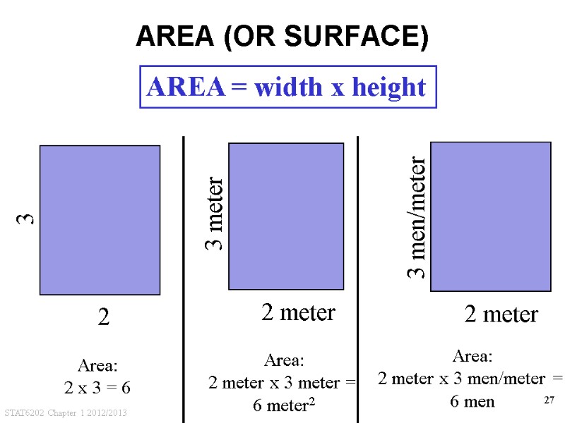
STAT6202 Chapter 1 2012/2013 27 AREA (OR SURFACE) Area: 2 x 3 = 6 Area: 2 meter x 3 meter = 6 meter2 Area: 2 meter x 3 men/meter = 6 men AREA = width x height

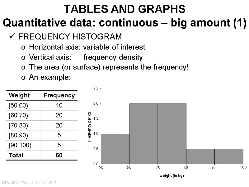
STAT6202 Chapter 1 2012/2013 28 TABLES AND GRAPHS Quantitative data: continuous – big amount (1) FREQUENCY HISTOGRAM Horizontal axis: variable of interest Vertical axis: frequency density The area (or surface) represents the frequency! An example:

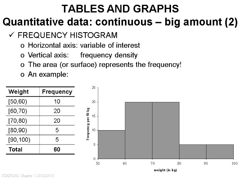
STAT6202 Chapter 1 2012/2013 29 TABLES AND GRAPHS Quantitative data: continuous – big amount (2) FREQUENCY HISTOGRAM Horizontal axis: variable of interest Vertical axis: frequency density The area (or surface) represents the frequency! An example:

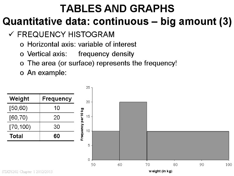
STAT6202 Chapter 1 2012/2013 30 TABLES AND GRAPHS Quantitative data: continuous – big amount (3) FREQUENCY HISTOGRAM Horizontal axis: variable of interest Vertical axis: frequency density The area (or surface) represents the frequency! An example:

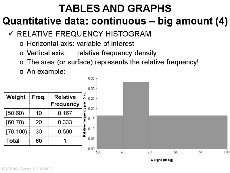
STAT6202 Chapter 1 2012/2013 31 TABLES AND GRAPHS Quantitative data: continuous – big amount (4) RELATIVE FREQUENCY HISTOGRAM Horizontal axis: variable of interest Vertical axis: relative frequency density The area (or surface) represents the relative frequency! An example:

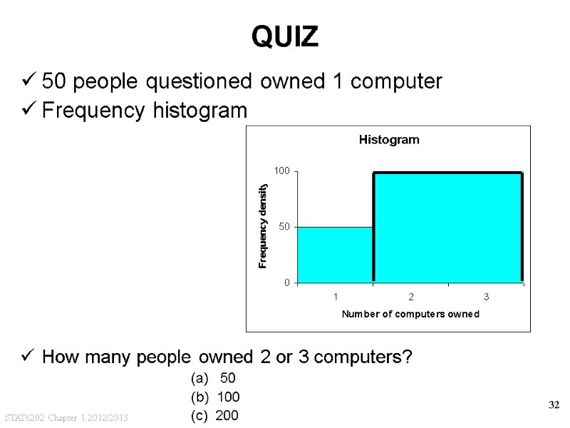
STAT6202 Chapter 1 2012/2013 32 QUIZ 50 people questioned owned 1 computer Frequency histogram How many people owned 2 or 3 computers? (a) 50 (b) 100 (c) 200

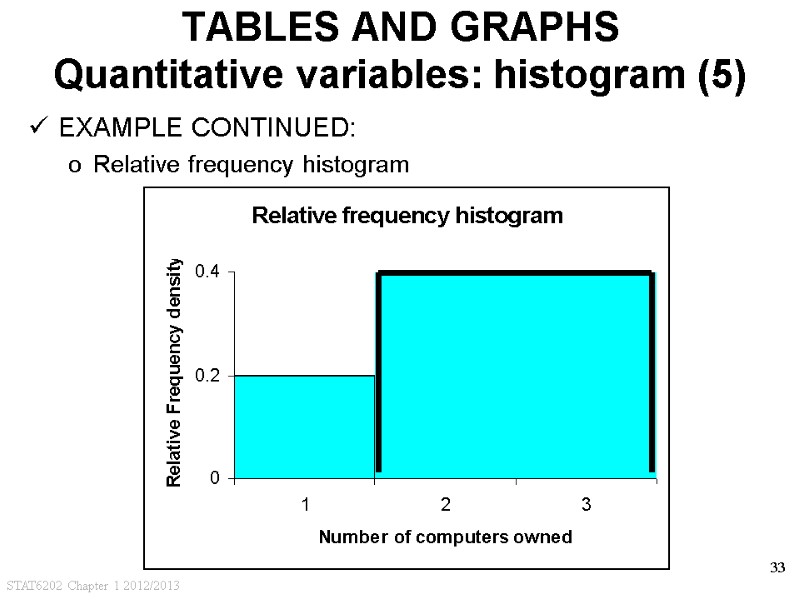
STAT6202 Chapter 1 2012/2013 33 TABLES AND GRAPHS Quantitative variables: histogram (5) EXAMPLE CONTINUED: Relative frequency histogram

STAT6202 Chapter 1 2012/2013 34 CHAPTER 1 Data summary and presentation POPULATION AND SAMPLES TYPES OF VARIABLES SUMMARY STATISTICS TABLES AND GRAPHS BOXPLOT AND SKEWNESS LINEAR TRANSFORMATIONS LOG TRANSFORMATIONS

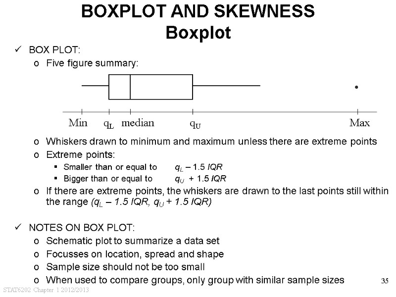
STAT6202 Chapter 1 2012/2013 35 BOXPLOT AND SKEWNESS Boxplot BOX PLOT: Five figure summary: Whiskers drawn to minimum and maximum unless there are extreme points Extreme points: Smaller than or equal to qL – 1.5 IQR Bigger than or equal to qU + 1.5 IQR If there are extreme points, the whiskers are drawn to the last points still within the range (qL – 1.5 IQR, qU + 1.5 IQR) NOTES ON BOX PLOT: Schematic plot to summarize a data set Focusses on location, spread and shape Sample size should not be too small When used to compare groups, only group with similar sample sizes

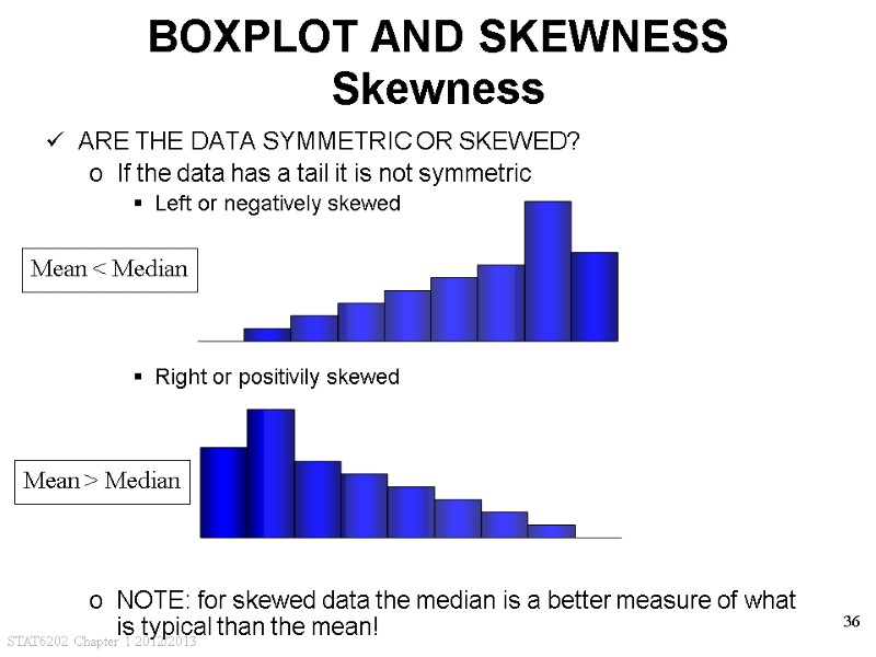
STAT6202 Chapter 1 2012/2013 36 BOXPLOT AND SKEWNESS Skewness ARE THE DATA SYMMETRIC OR SKEWED? If the data has a tail it is not symmetric Left or negatively skewed Right or positivily skewed NOTE: for skewed data the median is a better measure of what is typical than the mean! Mean < Median Mean > Median

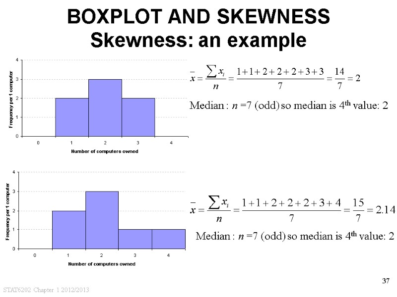
STAT6202 Chapter 1 2012/2013 37 BOXPLOT AND SKEWNESS Skewness: an example Median : n =7 (odd) so median is 4th value: 2 Median : n =7 (odd) so median is 4th value: 2

STAT6202 Chapter 1 2012/2013 38 DESCRIPTIVE STATISTICS What are we trying to do? DETECT MAIN DATA FEATURES AND PATTERNS Location, spread, shape Exception to the general pattern, e.g. outliers Comparison between groups (see appendix) Relationships between variables SUMMARIZE THE ESSENTIAL INFORMATION Often combination of text, summary statistics and graphs best PRESENT RESULTS INFORMATIVELY AND WITH INTEGRITY SEE THROUGH INADEQUATE AND MISLEADING PRESENTATION

STAT6202 Chapter 1 2012/2013 39 CHAPTER 1 Data summary and presentation POPULATION AND SAMPLES TYPES OF VARIABLES SUMMARY STATISTICS TABLES AND GRAPHS BOXPLOT AND SKEWNESS LINEAR TRANSFORMATIONS LOG TRANSFORMATIONS

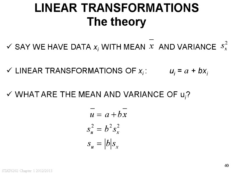
STAT6202 Chapter 1 2012/2013 40 LINEAR TRANSFORMATIONS The theory SAY WE HAVE DATA xi WITH MEAN AND VARIANCE LINEAR TRANSFORMATIONS OF xi : ui = a + bxi WHAT ARE THE MEAN AND VARIANCE OF ui?

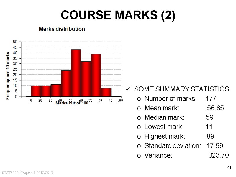
STAT6202 Chapter 1 2012/2013 41 COURSE MARKS (2) SOME SUMMARY STATISTICS: Number of marks: 177 Mean mark: 56.85 Median mark: 59 Lowest mark: 11 Highest mark: 89 Standard deviation: 17.99 Variance: 323.70

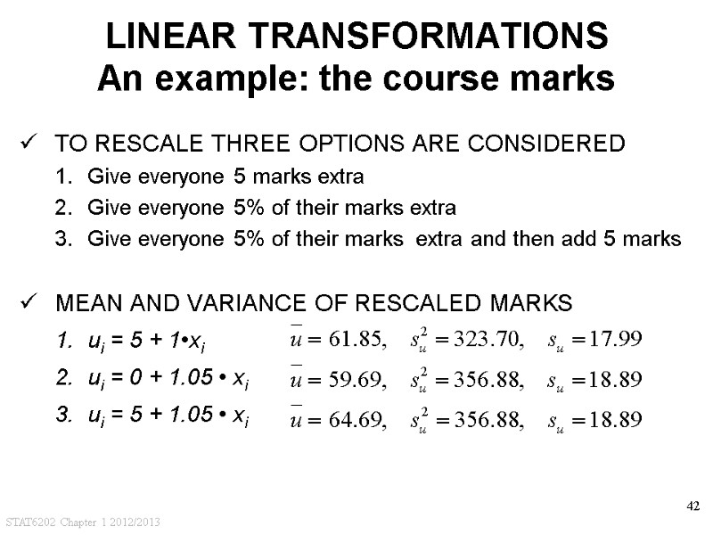
STAT6202 Chapter 1 2012/2013 42 LINEAR TRANSFORMATIONS An example: the course marks TO RESCALE THREE OPTIONS ARE CONSIDERED Give everyone 5 marks extra Give everyone 5% of their marks extra Give everyone 5% of their marks extra and then add 5 marks MEAN AND VARIANCE OF RESCALED MARKS ui = 5 + 1•xi ui = 0 + 1.05 • xi ui = 5 + 1.05 • xi

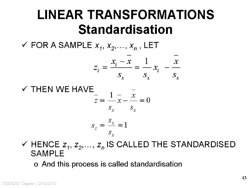
STAT6202 Chapter 1 2012/2013 43 LINEAR TRANSFORMATIONS Standardisation FOR A SAMPLE x1, x2,…, xn , LET THEN WE HAVE HENCE z1, z2,…, zn IS CALLED THE STANDARDISED SAMPLE And this process is called standardisation

STAT6202 Chapter 1 2012/2013 44 CHAPTER 1 Data summary and presentation POPULATION AND SAMPLES TYPES OF VARIABLES SUMMARY STATISTICS TABLES AND GRAPHS BOXPLOT AND SKEWNESS LINEAR TRANSFORMATIONS LOG TRANSFORMATIONS

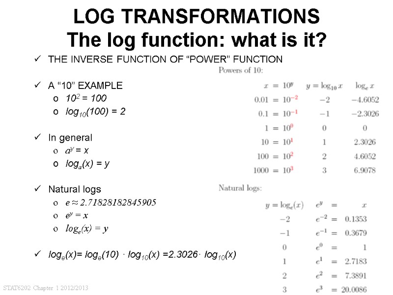
STAT6202 Chapter 1 2012/2013 45 LOG TRANSFORMATIONS The log function: what is it? THE INVERSE FUNCTION OF “POWER” FUNCTION A “10” EXAMPLE 102 = 100 log10(100) = 2 In general ay = x loga(x) = y Natural logs e ≈ 2.71828182845905 ey = x loge(x) = y loge(x)= loge(10) · log10(x) =2.3026· log10(x)

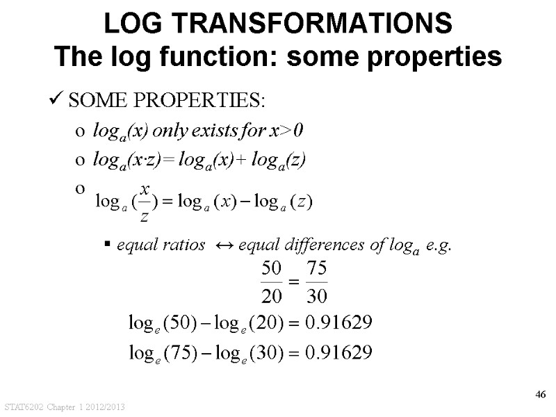
STAT6202 Chapter 1 2012/2013 46 LOG TRANSFORMATIONS The log function: some properties SOME PROPERTIES: loga(x) only exists for x>0 loga(x·z)= loga(x)+ loga(z) equal ratios ↔ equal differences of loga e.g.

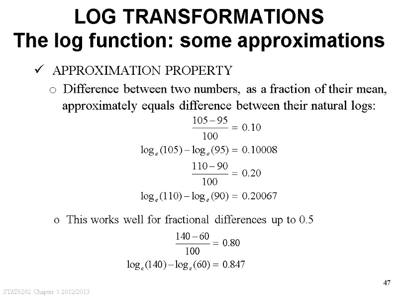
STAT6202 Chapter 1 2012/2013 47 LOG TRANSFORMATIONS The log function: some approximations APPROXIMATION PROPERTY o Difference between two numbers, as a fraction of their mean, approximately equals difference between their natural logs: This works well for fractional differences up to 0.5

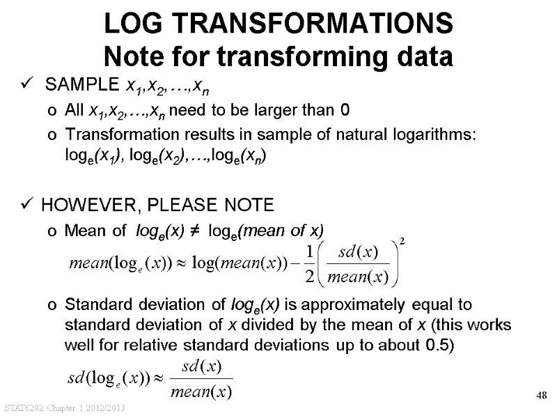
STAT6202 Chapter 1 2012/2013 48 SAMPLE x1,x2,…,xn All x1,x2,…,xn need to be larger than 0 Transformation results in sample of natural logarithms: loge(x1), loge(x2),…,loge(xn) HOWEVER, PLEASE NOTE Mean of loge(x) ≠ loge(mean of x) Standard deviation of loge(x) is approximately equal to standard deviation of x divided by the mean of x (this works well for relative standard deviations up to about 0.5) LOG TRANSFORMATIONS Note for transforming data

STAT6202 Chapter 1 2012/2013 49 APPENDIX Comparing groups back

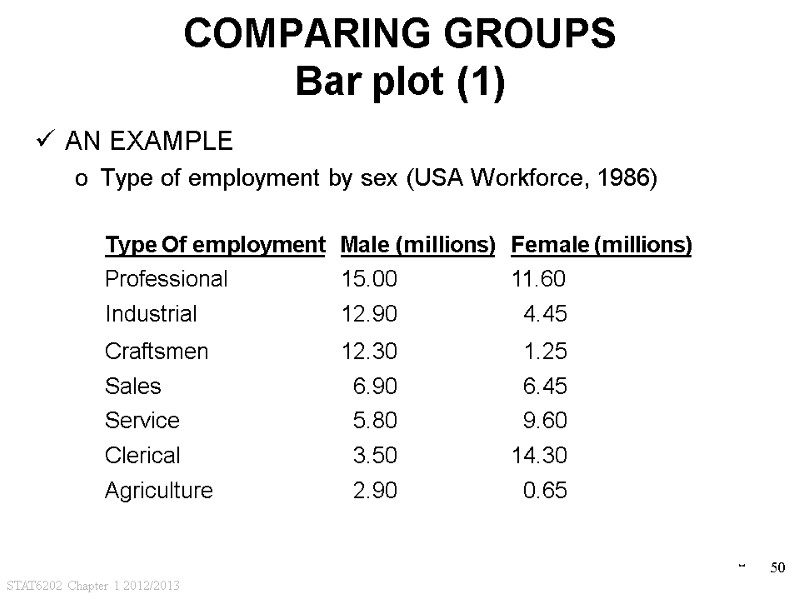
STAT6202 Chapter 1 2012/2013 50 COMPARING GROUPS Bar plot (1) AN EXAMPLE Type of employment by sex (USA Workforce, 1986) back

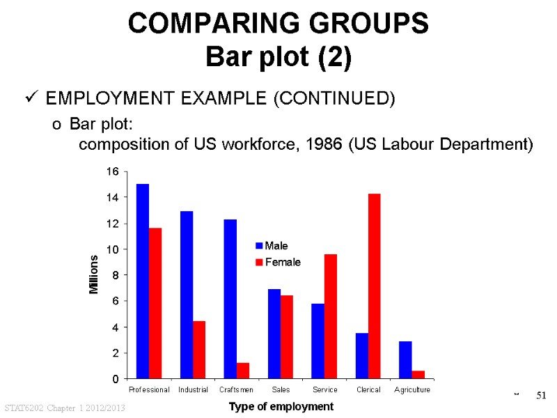
STAT6202 Chapter 1 2012/2013 51 COMPARING GROUPS Bar plot (2) EMPLOYMENT EXAMPLE (CONTINUED) Bar plot: composition of US workforce, 1986 (US Labour Department) back

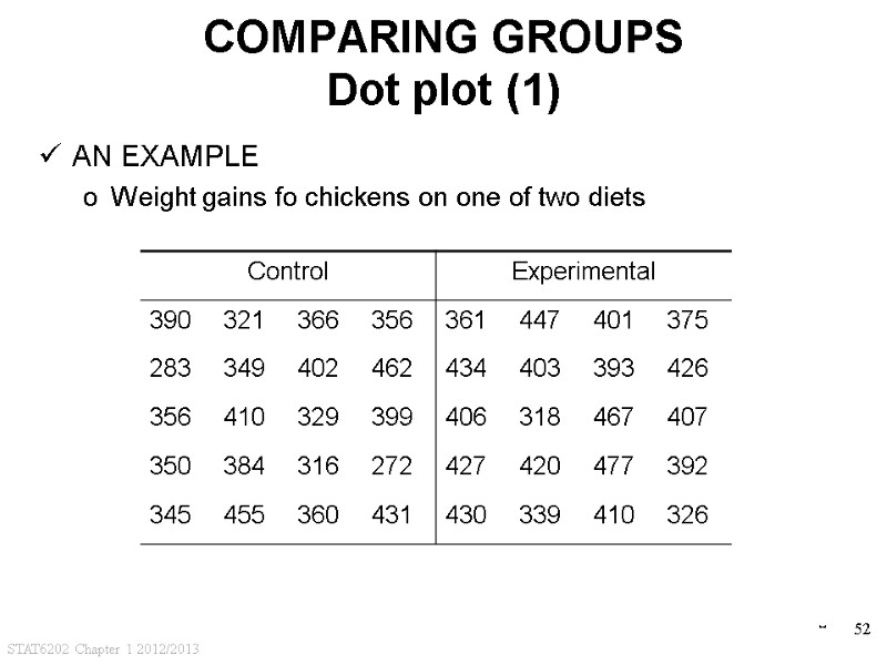
STAT6202 Chapter 1 2012/2013 52 COMPARING GROUPS Dot plot (1) AN EXAMPLE Weight gains fo chickens on one of two diets back

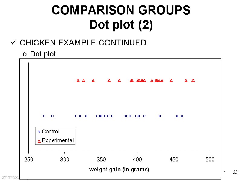
STAT6202 Chapter 1 2012/2013 53 COMPARISON GROUPS Dot plot (2) CHICKEN EXAMPLE CONTINUED Dot plot back

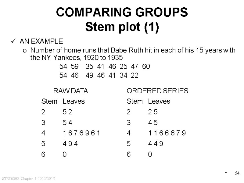
STAT6202 Chapter 1 2012/2013 54 COMPARING GROUPS Stem plot (1) AN EXAMPLE Number of home runs that Babe Ruth hit in each of his 15 years with the NY Yankees, 1920 to 1935 54 59 35 41 46 25 47 60 54 46 49 46 41 34 22 back

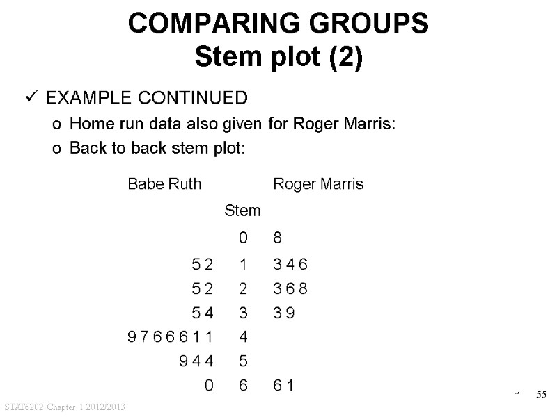
STAT6202 Chapter 1 2012/2013 55 COMPARING GROUPS Stem plot (2) EXAMPLE CONTINUED Home run data also given for Roger Marris: Back to back stem plot: back

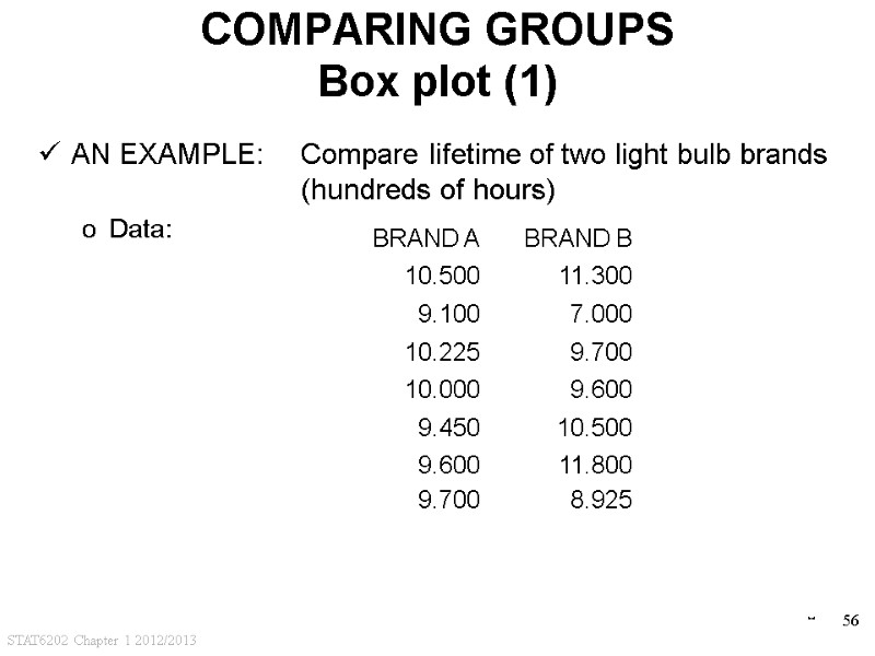
STAT6202 Chapter 1 2012/2013 56 COMPARING GROUPS Box plot (1) AN EXAMPLE: Compare lifetime of two light bulb brands (hundreds of hours) Data: back

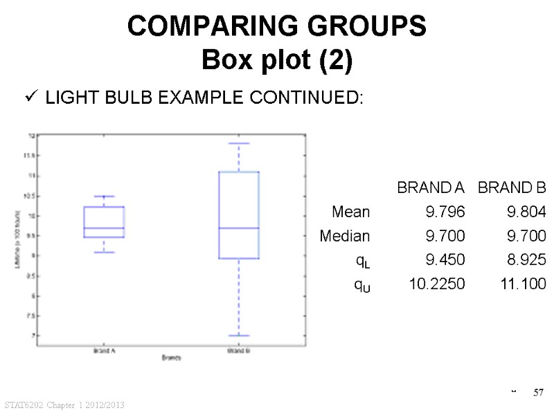
STAT6202 Chapter 1 2012/2013 57 COMPARING GROUPS Box plot (2) LIGHT BULB EXAMPLE CONTINUED: back