SECTION 8 FIELDS • Fields (functions)

SECTION 8 FIELDS

• Fields (functions) allow the creation and modification of a multitude of data sets. Data fields are used in the following modeling areas: – Loads and boundary conditions – Material properties – Element properties • Field input can either be tabular or continuous functions, with the input being scalar or vector. • Complex (number) scalar fields are also permitted if the Nastran analysis preference is used. – This allows, for example, real/imaginary or magnitude/phase components of a frequency dependent function to be defined. FIELDS

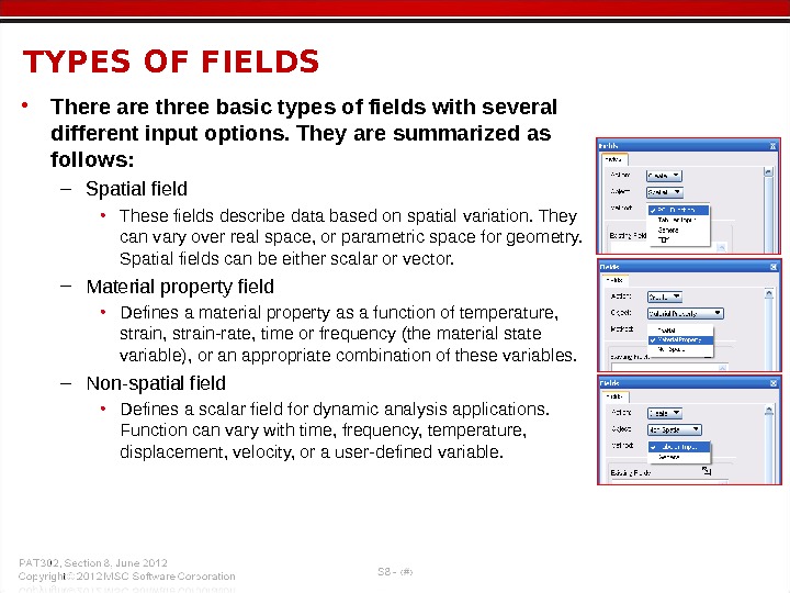
• There are three basic types of fields with several different input options. They are summarized as follows: – Spatial field • These fields describe data based on spatial variation. They can vary over real space, or parametric space for geometry. Spatial fields can be either scalar or vector. – Material property field • Defines a material property as a function of temperature, strain, strain-rate, time or frequency (the material state variable), or an appropriate combination of these variables. – Non-spatial field • Defines a scalar field for dynamic analysis applications. Function can vary with time, frequency, temperature, displacement, velocity, or a user-defined variable. TYPES OF FIELDS

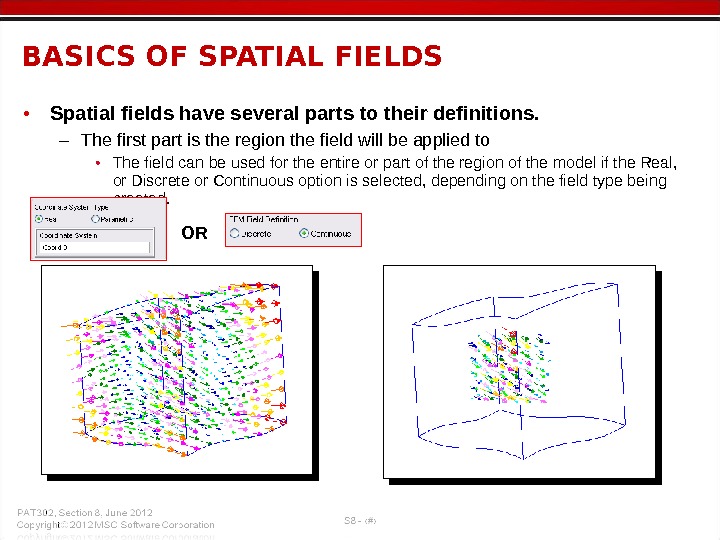
• Spatial fields have several parts to their definitions. – The first part is the region the field will be applied to • The field can be used for the entire or part of the region of the model if the Real, or Discrete or Continuous option is selected, depending on the field type being created. BASICS OF SPATIAL FIELDS OR

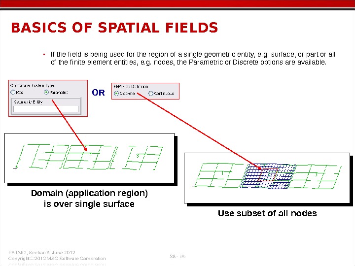
• If the field is being used for the region of a single geometric entity, e. g. surface, or part or all of the finite element entities, e. g. nodes, the Parametric or Discrete options are available. BASICS OF SPATIAL FIELDS Use subset of all nodes. Domain (application region) is over single surface OR

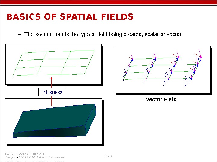
– The second part is the type of field being created, scalar or vector. BASICS OF SPATIAL FIELDS Vector Field. Thickness

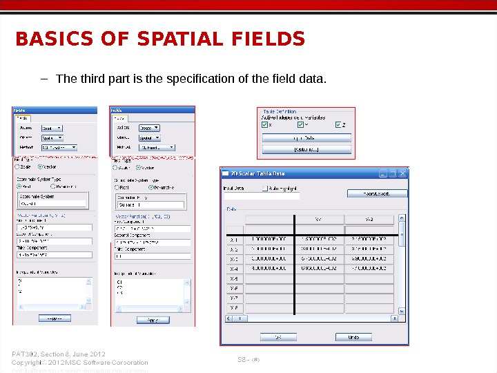
– The third part is the specification of the field data. BASICS OF SPATIAL FIELDS

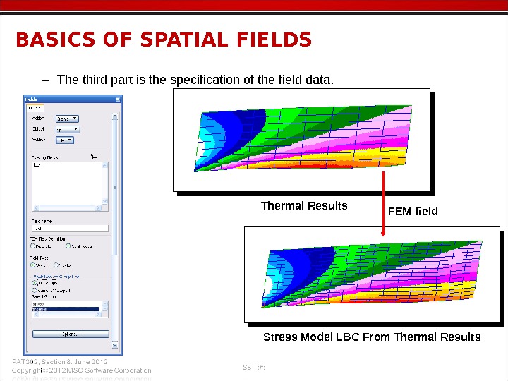
– The third part is the specification of the field data. BASICS OF SPATIAL FIELDS Thermal Results FEM field Stress Model LBC From Thermal Results

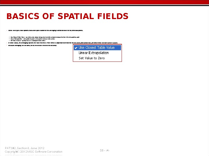
BASICS OF SPATIAL FIELDS • Some field types have options that allow specification of the averaging method between or beyond data points. – Use Closest Table Value – use table value whose independent variable value(s) is closest to that of the interpolation point – Linear Extrapolation – extrapolate beyond or interpolate between table entries – Set Value to Zero – specify data as zero beyond table entries • In some cases, the averaging options will have no effect. Their effect is dependent on how the field is used, and sometimes, on which finite element solver is used. • Because averaging will be done, fields need to be checked for accuracy.

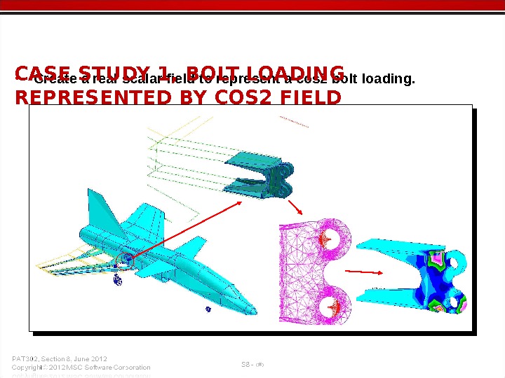
• Create a real scalar field to represent a cos 2 bolt loading. CASE STUDY 1, BOLT LOADING REPRESENTED BY COS 2 FIEL

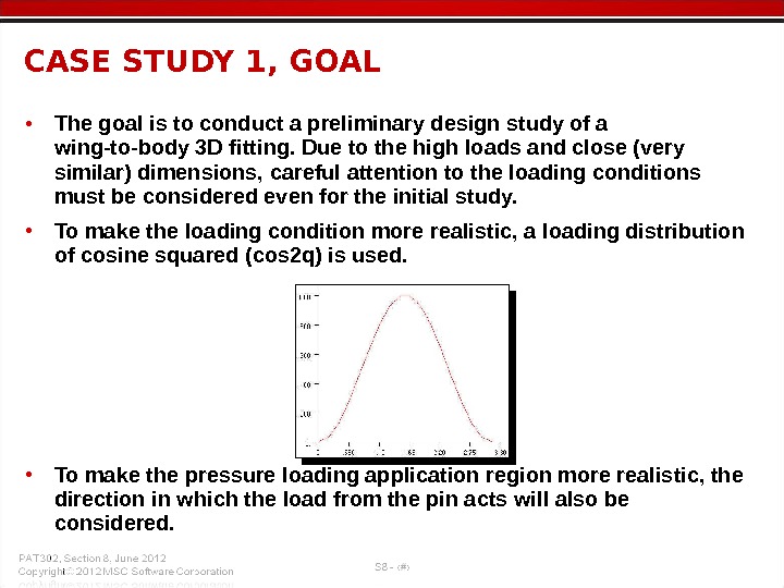
• The goal is to conduct a preliminary design study of a wing-to-body 3 D fitting. Due to the high loads and close (very similar) dimensions, careful attention to the loading conditions must be considered even for the initial study. • To make the loading condition more realistic, a loading distribution of cosine squared (cos 2 q) is used. • To make the pressure loading application region more realistic, the direction in which the load from the pin acts will also be considered. CASE STUDY 1, GOAL

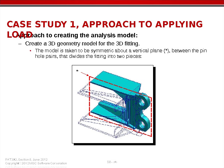
• Approach to creating the analysis model: – Create a 3 D geometry model for the 3 D fitting. • The model is taken to be symmetric about a vertical plane (*), between the pin hole pairs, that divides the fitting into two pieces: CASE STUDY 1, APPROACH TO APPLYING LOAD *

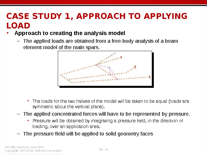
CASE STUDY 1, APPROACH TO APPLYING LOAD • Approach to creating the analysis model – The applied loads are obtained from a free-body analysis of a beam element model of the main spars. • The loads for the two halves of the model will be taken to be equal (loads are symmetric about the vertical plane). – The applied concentrated forces will have to be represented by pressure. • Pressure will be obtained by integrating a pressure field, in the direction of loading, over an application area. – The pressure field will be applied to solid geometry faces

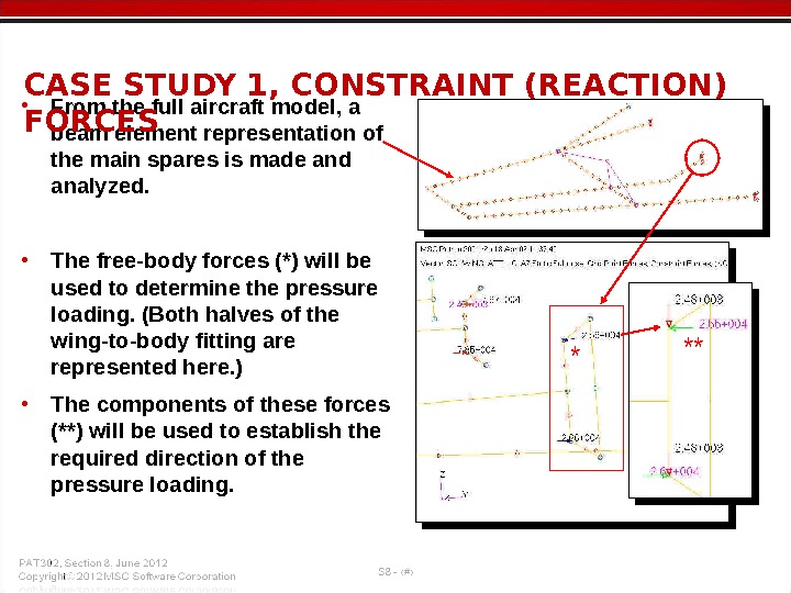
• From the full aircraft model, a beam element representation of the main spares is made and analyzed. • The free-body forces (*) will be used to determine the pressure loading. (Both halves of the wing-to-body fitting are represented here. ) • The components of these forces (**) will be used to establish the required direction of the pressure loading. CASE STUDY 1, CONSTRAINT (REACTION) FORCES * **

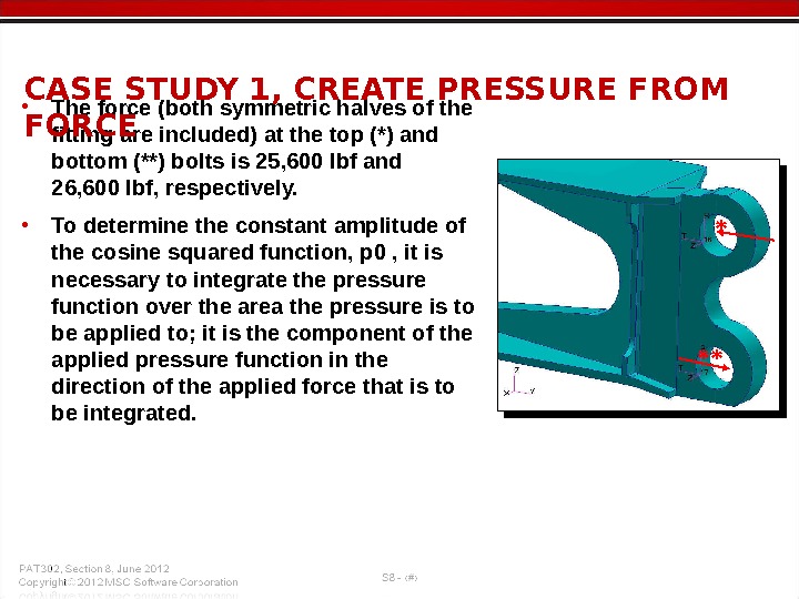
• The force (both symmetric halves of the fitting are included) at the top (*) and bottom (**) bolts is 25, 600 lbf and 26, 600 lbf, respectively. • To determine the constant amplitude of the cosine squared function, p 0 , it is necessary to integrate the pressure function over the area the pressure is to be applied to; it is the component of the applied pressure function in the direction of the applied force that is to be integrated. CASE STUDY 1, CREATE PRESSURE FROM FORCE ** *

Rtp 34 Rtd θπ/2)sin(θ)( θcospf 02π 0 0 2 Dt 3 f 4 Rt 3 f p 0 psi 5. 13052 )980. 0*2(*501. 1*2 25600*3 2 Dt 3 f p 0 π/2)( θcospp 2 0 • Integrating the component of the pressure function, in the direction of the applied load, the following is found: where R is the radius of the bolt hole, and t is the thickness of the clevis. • Solve for p 0 in terms of the applied concentrated load • Applying this formula to one of the applied forces, the following is found: where D = 1. 501 in and t = 0. 980 in. ; multiply t by 2 for symmetry. CASE STUDY 1, CREATE PRESSURE FROM FOR

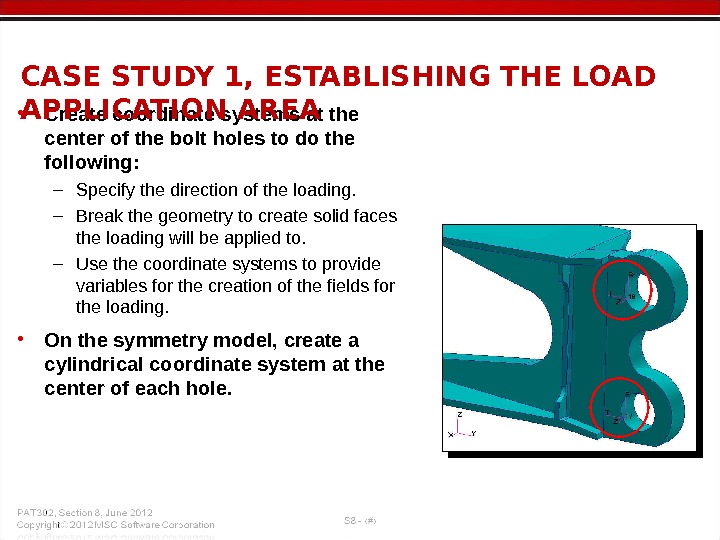
• Create coordinate systems at the center of the bolt holes to do the following: – Specify the direction of the loading. – Break the geometry to create solid faces the loading will be applied to. – Use the coordinate systems to provide variables for the creation of the fields for the loading. • On the symmetry model, create a cylindrical coordinate system at the center of each hole. CASE STUDY 1, ESTABLISHING THE LOAD APPLICATION AR

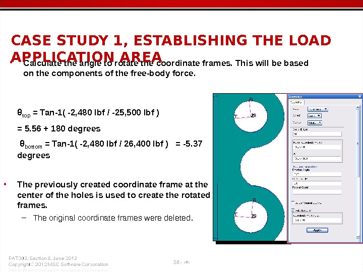
• Calculate the angle to rotate the coordinate frames. This will be based on the components of the free-body force. CASE STUDY 1, ESTABLISHING THE LOAD APPLICATION AREA θ top = Tan-1( -2, 480 lbf / -25, 500 lbf ) = 5. 56 + 180 degrees θ bottom = Tan-1( -2, 480 lbf / 26, 400 lbf ) = -5. 37 degrees • The previously created coordinate frame at the center of the holes is used to create the rotated frames. – The original coordinate frames were deleted.

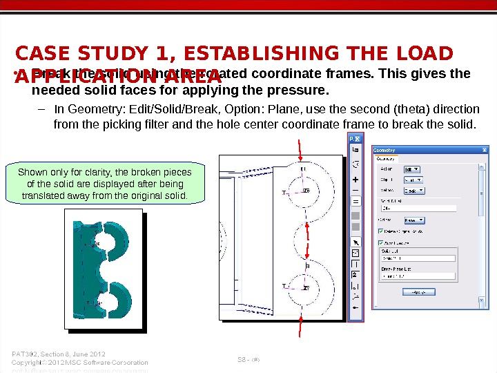
• Break the solid using the rotated coordinate frames. This gives the needed solid faces for applying the pressure. – In Geometry: Edit/Solid/Break, Option: Plane, use the second (theta) direction from the picking filter and the hole center coordinate frame to break the solid. CASE STUDY 1, ESTABLISHING THE LOAD APPLICATION AREA Shown only for clarity, the broken pieces of the solid are displayed after being translated away from the original solid.

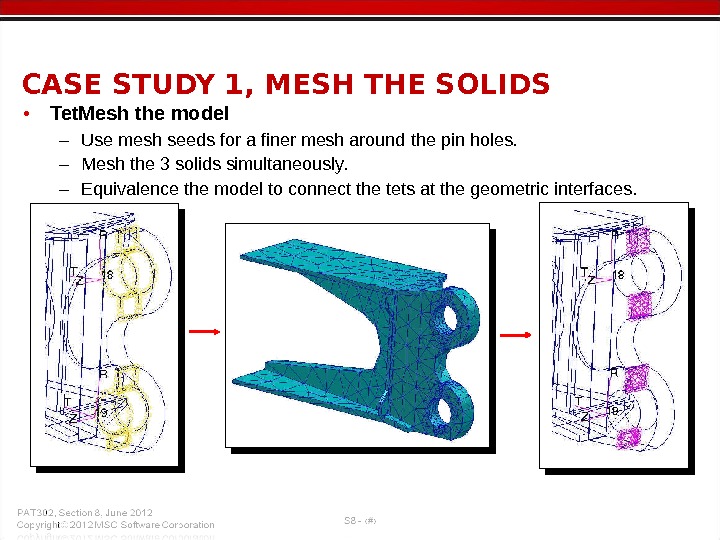
• Tet. Mesh the model – Use mesh seeds for a finer mesh around the pin holes. – Mesh the 3 solids simultaneously. – Equivalence the model to connect the tets at the geometric interfaces. CASE STUDY 1, MESH THE SOLIDS

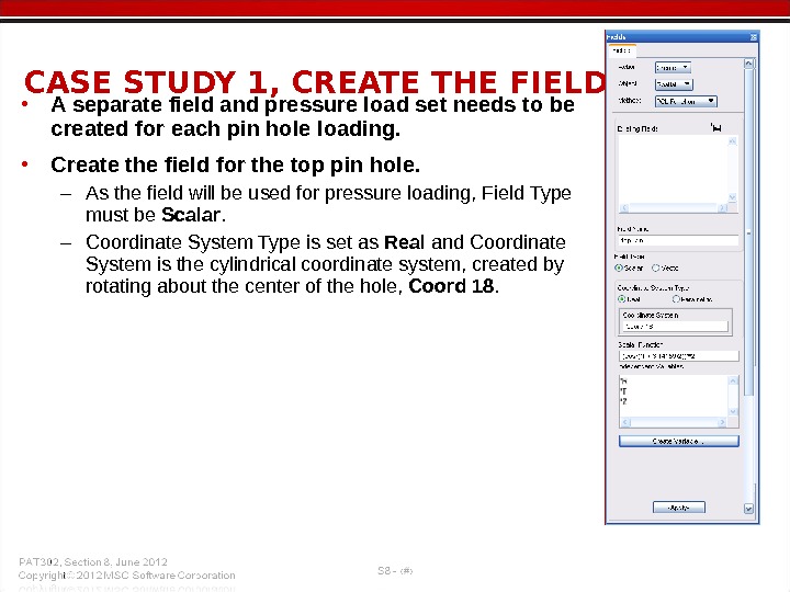
• A separate field and pressure load set needs to be created for each pin hole loading. • Create the field for the top pin hole. – As the field will be used for pressure loading, Field Type must be Scalar. – Coordinate System Type is set as Real and Coordinate System is the cylindrical coordinate system, created by rotating about the center of the hole, Coord 18. CASE STUDY 1, CREATE THE FIEL

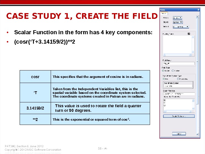
cosr This specifies that the argument of cosine is in radians. ‘ T Taken from the Independent Variables list, this is the spatial variable based on the coordinate system selected. The coordinate systems created in Patran are in radians. 3. 14159/2 This value is used to rotate the field a quarter turn or 90 degrees. **2 This is the exponential or squared term of cos 2. • Scalar Function in the form has 4 key components: • (cosr(‘T+3. 14159/2))**2 CASE STUDY 1, CREATE THE FIEL

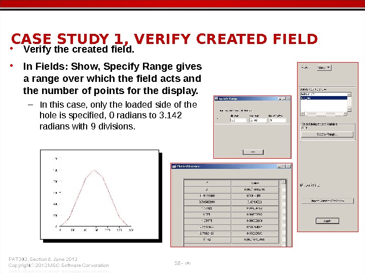
• Verify the created field. • In Fields: Show, Specify Range gives a range over which the field acts and the number of points for the display. – In this case, only the loaded side of the hole is specified, 0 radians to 3. 142 radians with 9 divisions. CASE STUDY 1, VERIFY CREATED FIEL

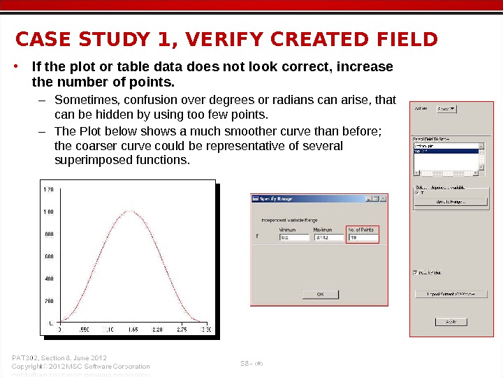
• If the plot or table data does not look correct, increase the number of points. – Sometimes, confusion over degrees or radians can arise, that can be hidden by using too few points. – The Plot below shows a much smoother curve than before; the coarser curve could be representative of several superimposed functions. CASE STUDY 1, VERIFY CREATED FIEL

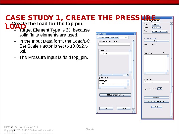
• Create the load for the top pin. – Target Element Type is 3 D because solid finite elements are used. – In the Input Data form, the Load/BC Set Scale Factor is set to 13, 052. 5 psi. – The Pressure input is field top_pin. CASE STUDY 1, CREATE THE PRESSURE LO

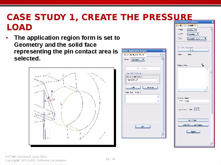
• The application region form is set to Geometry and the solid face representing the pin contact area is selected. CASE STUDY 1, CREATE THE PRESSURE LO

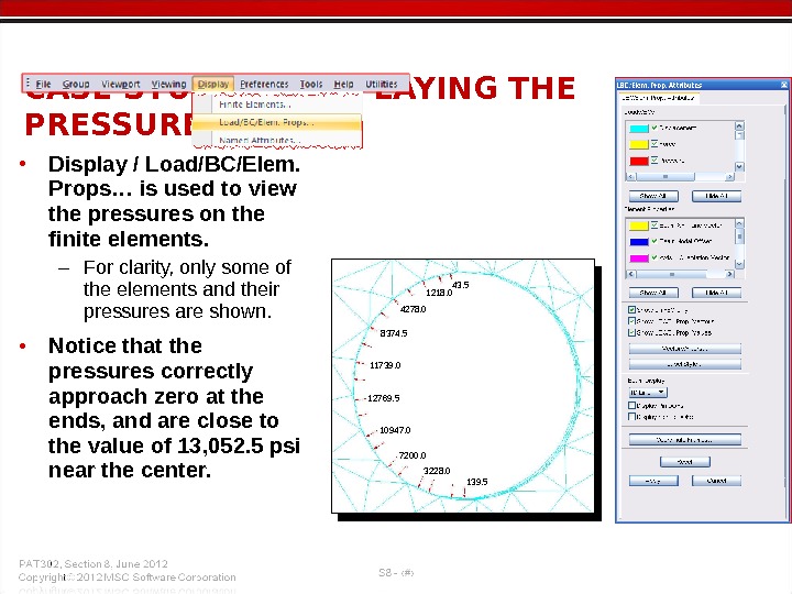
• Display / Load/BC/Elem. Props… is used to view the pressures on the finite elements. – For clarity, only some of the elements and their pressures are shown. • Notice that the pressures correctly approach zero at the ends, and are close to the value of 13, 052. 5 psi near the center. CASE STUDY 1, DISPLAYING THE PRESSURE LOAD 43. 5 1218. 0 4278. 0 8374. 5 11739. 0 12769. 5 10947. 0 7200. 0 3228. 0 139.

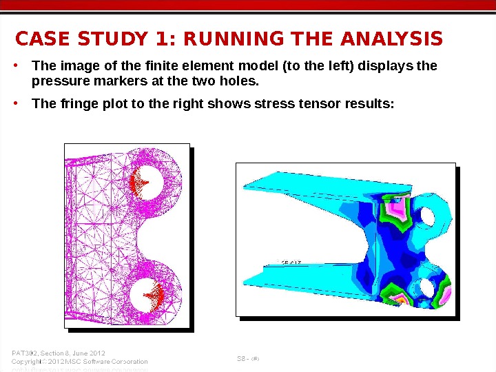
• The image of the finite element model (to the left) displays the pressure markers at the two holes. • The fringe plot to the right shows stress tensor results: CASE STUDY 1: RUNNING THE ANALYSIS

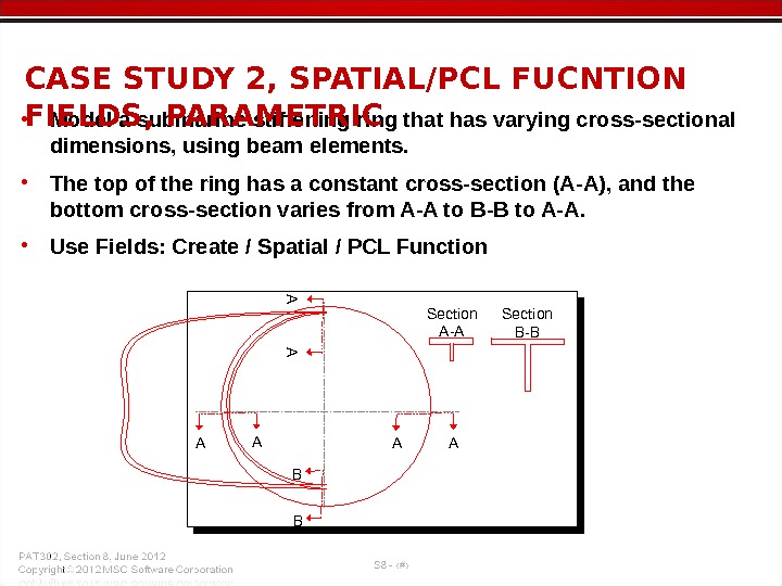
• Model a submarine stiffening ring that has varying cross-sectional dimensions, using beam elements. • The top of the ring has a constant cross-section (A-A), and the bottom cross-section varies from A-A to B-B to A-A. • Use Fields: Create / Spatial / PCL Function CASE STUDY 2, SPATIAL/PCL FUCNTION FIELDS, PARAMETRIC Section A-A Section B-

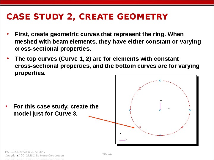
• First, create geometric curves that represent the ring. When meshed with beam elements, they have either constant or varying cross-sectional properties. • The top curves (Curve 1, 2) are for elements with constant cross-sectional properties, and the bottom curves are for varying properties. CASE STUDY 2, CREATE GEOMETRY • For this case study, create the model just for Curve 3.

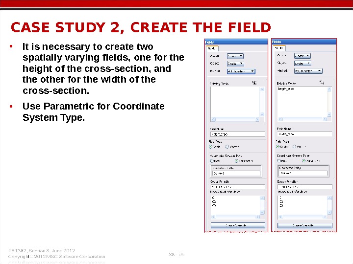
• It is necessary to create two spatially varying fields, one for the height of the cross-section, and the other for the width of the cross-section. • Use Parametric for Coordinate System Type. CASE STUDY 2, CREATE THE FIEL

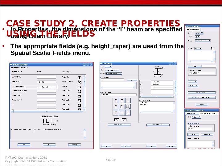
• In Properties, the dimensions of the “I” beam are specified using Beam Library. • The appropriate fields (e. g. height_taper) are used from the Spatial Scalar Fields menu. CASE STUDY 2, CREATE PROPERTIES USING THE FIELDS

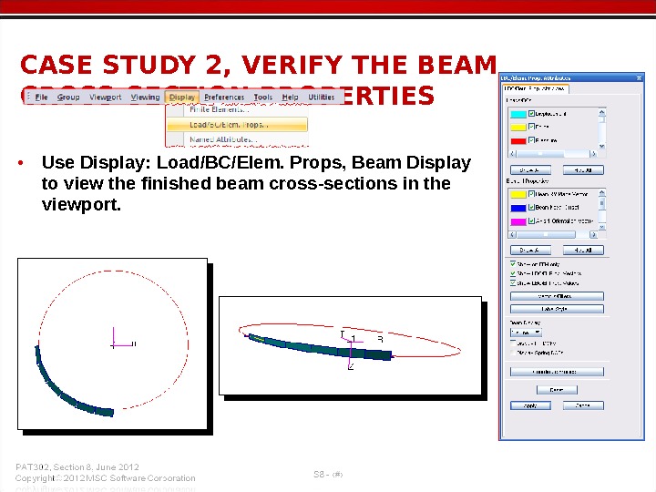
• Use Display: Load/BC/Elem. Props, Beam Display to view the finished beam cross-sections in the viewport. CASE STUDY 2, VERIFY THE BEAM CROSS-SECTION PROPERTIES

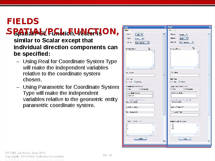
• Spatial/PCL Function, Vector is similar to Scalar except that individual direction components can be specified: – Using Real for Coordinate System Type will make the independent variables relative to the coordinate system chosen. – Using Parametric for Coordinate System Type will make the independent variables relative to the geometric entity parametric coordinate system. FIELDS SPATIAL/PCL FUNCTION, VECTOR

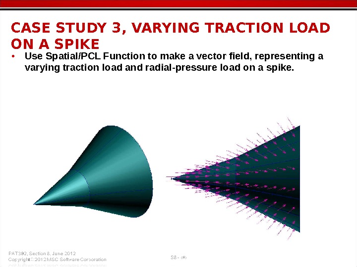
• Use Spatial/PCL Function to make a vector field, representing a varying traction load and radial-pressure load on a spike. CASE STUDY 3, VARYING TRACTION LOAD ON A SPIK

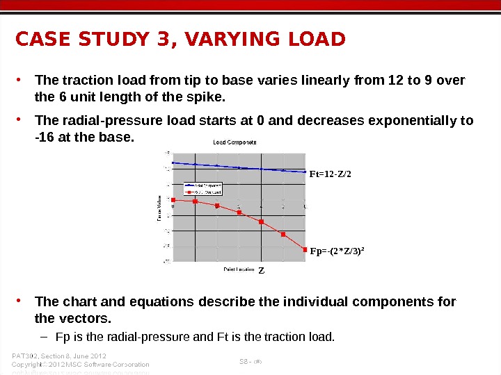
Ft=12 -Z/2 Fp=-(2*Z/3) 2 Z • The traction load from tip to base varies linearly from 12 to 9 over the 6 unit length of the spike. • The radial-pressure load starts at 0 and decreases exponentially to -16 at the base. • The chart and equations describe the individual components for the vectors. – Fp is the radial-pressure and Ft is the traction load. CASE STUDY 3, VARYING LO

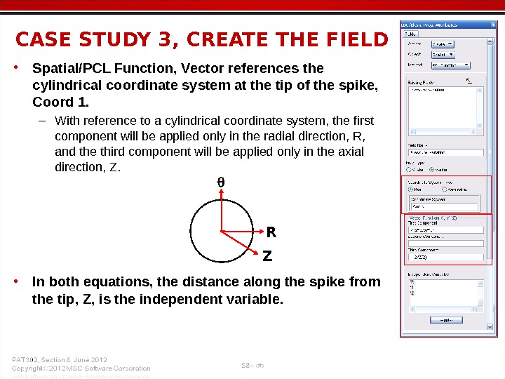
Z R • Spatial/PCL Function, Vector references the cylindrical coordinate system at the tip of the spike, Coord 1. – With reference to a cylindrical coordinate system, the first component will be applied only in the radial direction, R, and the third component will be applied only in the axial direction, Z. • In both equations, the distance along the spike from the tip, Z, is the independent variable. CASE STUDY 3, CREATE THE FIEL

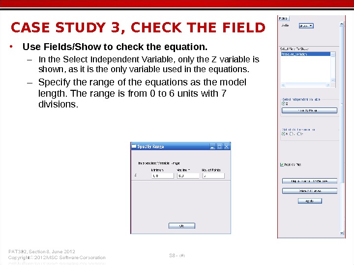
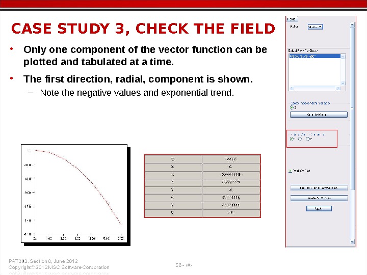
• Use Fields/Show to check the equation. – In the Select Independent Variable, only the Z variable is shown, as it is the only variable used in the equations. – Specify the range of the equations as the model length. The range is from 0 to 6 units with 7 divisions. CASE STUDY 3, CHECK THE FIEL

• Only one component of the vector function can be plotted and tabulated at a time. • The first direction, radial, component is shown. – Note the negative values and exponential trend. CASE STUDY 3, CHECK THE FIEL

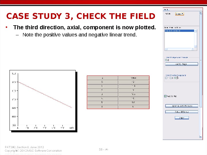
• The third direction, axial, component is now plotted. – Note the positive values and negative linear trend. CASE STUDY 3, CHECK THE FIEL

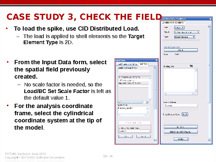
• To load the spike, use CID Distributed Load. – The load is applied to shell elements so the Target Element Type is 2 D. CASE STUDY 3, CHECK THE FIELD • From the Input Data form, select the spatial field previously created. – No scale factor is needed, so the Load/BC Set Scale Factor is left as the default value 1. • For the analysis coordinate frame, select the cylindrical coordinate system at the tip of the model.

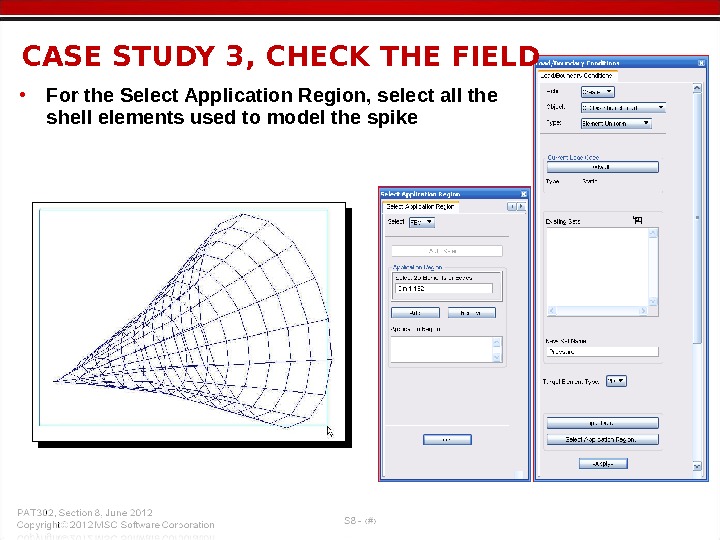
• For the Select Application Region, select all the shell elements used to model the spike. CASE STUDY 3, CHECK THE FIEL

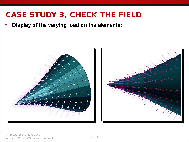
• Display of the varying load on the elements: CASE STUDY 3, CHECK THE FIEL

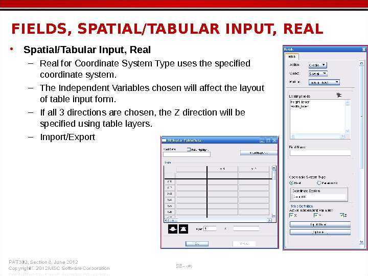
• Spatial/Tabular Input, Real – Real for Coordinate System Type uses the specified coordinate system. – The Independent Variables chosen will affect the layout of table input form. – If all 3 directions are chosen, the Z direction will be specified using table layers. – Import/Export. FIELDS, SPATIAL/TABULAR INPUT, REAL

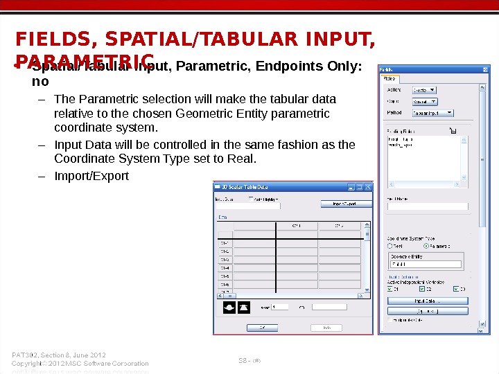
• Spatial/Tabular Input, Parametric, Endpoints Only: no – The Parametric selection will make the tabular data relative to the chosen Geometric Entity parametric coordinate system. – Input Data will be controlled in the same fashion as the Coordinate System Type set to Real. – Import/Export. FIELDS, SPATIAL/TABULAR INPUT, PARAMETRI

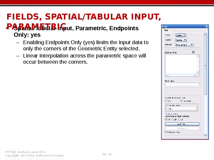
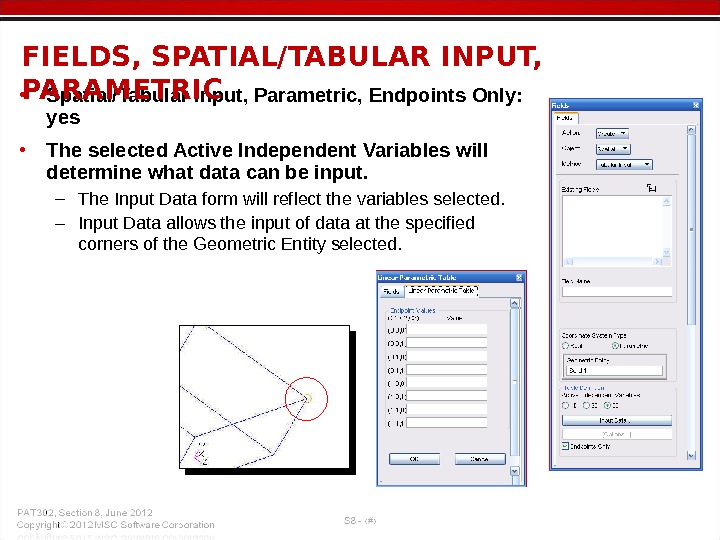
• Spatial/Tabular Input, Parametric, Endpoints Only: yes – Enabling Endpoints Only (yes) limits the input data to only the corners of the Geometric Entity selected. – Linear interpolation across the parametric space will occur between the corners. FIELDS, SPATIAL/TABULAR INPUT, PARAMETRI

• Spatial/Tabular Input, Parametric, Endpoints Only: yes • The selected Active Independent Variables will determine what data can be input. – The Input Data form will reflect the variables selected. – Input Data allows the input of data at the specified corners of the Geometric Entity selected. FIELDS, SPATIAL/TABULAR INPUT, PARAMETRI

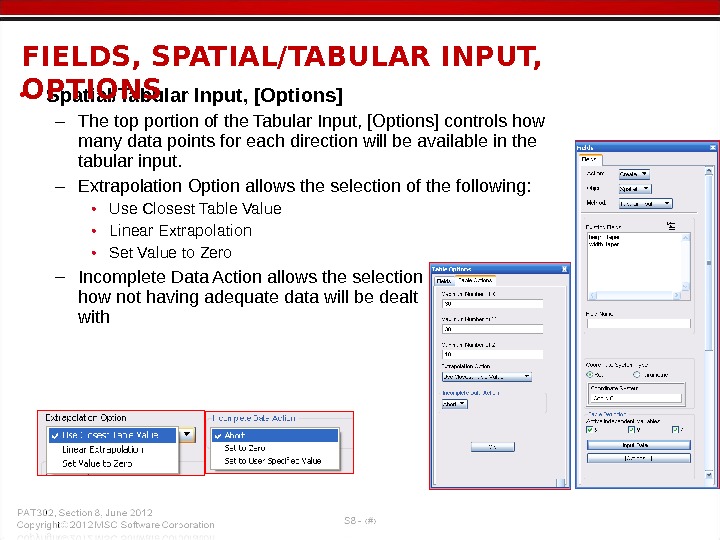
• Spatial/Tabular Input, [Options] – The top portion of the Tabular Input, [Options] controls how many data points for each direction will be available in the tabular input. – Extrapolation Option allows the selection of the following: • Use Closest Table Value • Linear Extrapolation • Set Value to Zero – Incomplete Data Action allows the selection of how not having adequate data will be dealt with. FIELDS, SPATIAL/TABULAR INPUT, OPTIONS

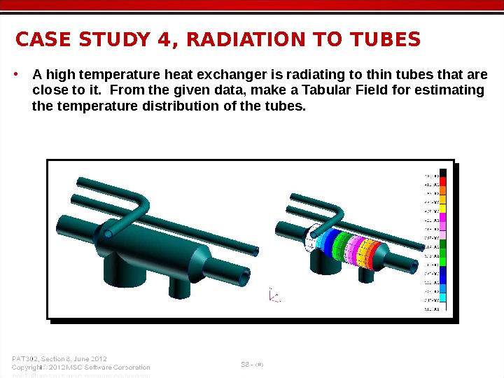
• A high temperature heat exchanger is radiating to thin tubes that are close to it. From the given data, make a Tabular Field for estimating the temperature distribution of the tubes. CASE STUDY 4, RADIATION TO TUBES

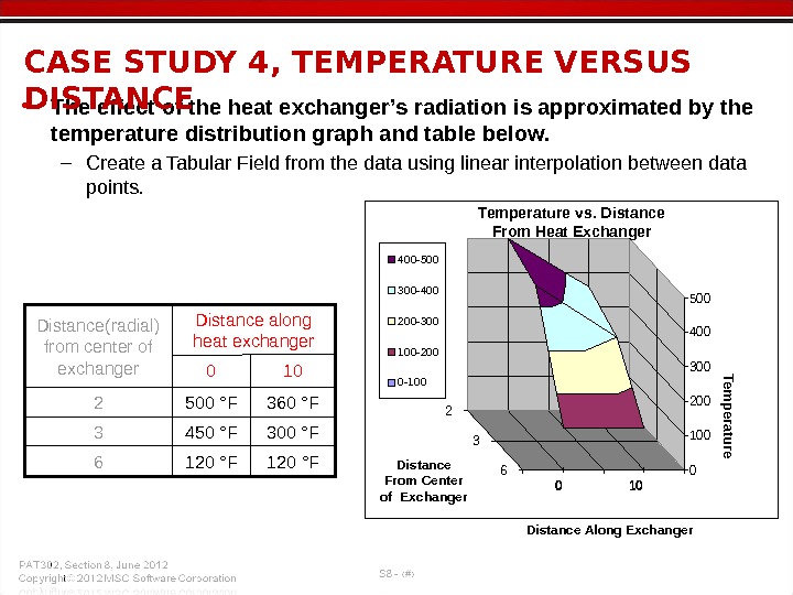
0 100 200 300 400 500 2 3 6 400 -500 300 -400 200 -300 100 -200 0 -100 Distance Along Exchanger. Distance From Center of Exchanger Tem perature Temperature vs. Distance From Heat Exchanger Distance along heat exchanger. Distance(radial) from center of exchanger 120 °F 6 300 °F 450 °F 3 360 °F 500 °F 2 100 • The effect of the heat exchanger’s radiation is approximated by the temperature distribution graph and table below. – Create a Tabular Field from the data using linear interpolation between data points. CASE STUDY 4, TEMPERATURE VERSUS DISTAN

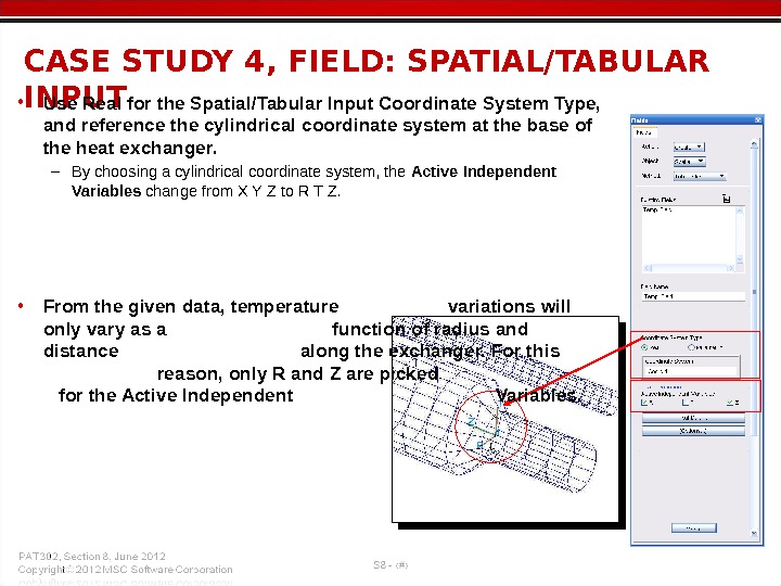
CASE STUDY 4, FIELD: SPATIAL/TABULAR INPUT • Use Real for the Spatial/Tabular Input Coordinate System Type, and reference the cylindrical coordinate system at the base of the heat exchanger. – By choosing a cylindrical coordinate system, the Active Independent Variables change from X Y Z to R T Z. • From the given data, temperature variations will only vary as a function of radius and distance along the exchanger. For this reason, only R and Z are picked for the Active Independent Variables.

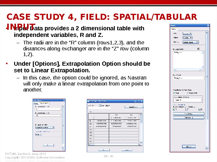
• Input Data provides a 2 dimensional table with independent variables, R and Z. – The radii are in the “R” column (rows 1, 2, 3), and the distances along exchanger are in the “Z” row (column 1, 2). • Under [Options], Extrapolation Option should be set to Linear Extrapolation. – In this case, the option could be ignored, as Nastran will only make a linear extrapolation from one point to another. CASE STUDY 4, FIELD: SPATIAL/TABULAR INPUT

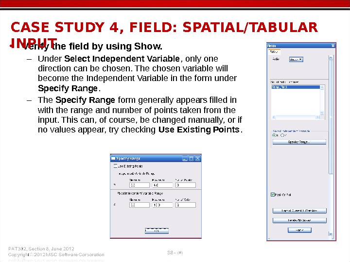
• Verify the field by using Show. – Under Select Independent Variable , only one direction can be chosen. The chosen variable will become the Independent Variable in the form under Specify Range. – The Specify Range form generally appears filled in with the range and number of points taken from the input. This can, of course, be changed manually, or if no values appear, try checking Use Existing Points. CASE STUDY 4, FIELD: SPATIAL/TABULAR INPUT

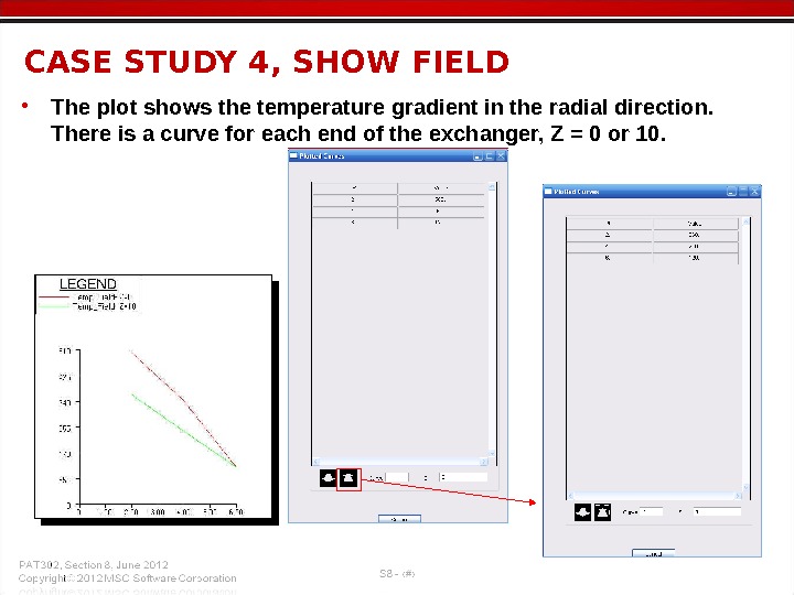
• The plot shows the temperature gradient in the radial direction. There is a curve for each end of the exchanger, Z = 0 or 10. CASE STUDY 4, SHOW FIEL

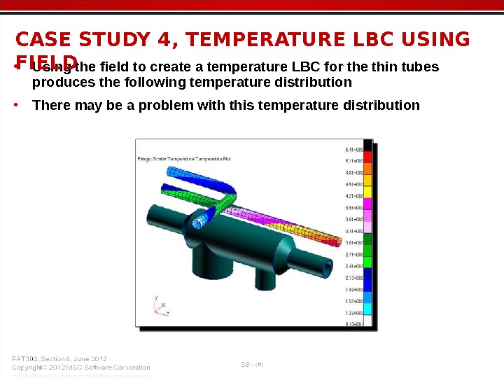
• Using the field to create a temperature LBC for the thin tubes produces the following temperature distribution • There may be a problem with this temperature distribution. CASE STUDY 4, TEMPERATURE LBC USING FIEL

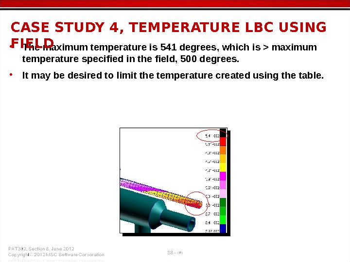
• The maximum temperature is 541 degrees, which is > maximum temperature specified in the field, 500 degrees. • It may be desired to limit the temperature created using the table. CASE STUDY 4, TEMPERATURE LBC USING FIEL

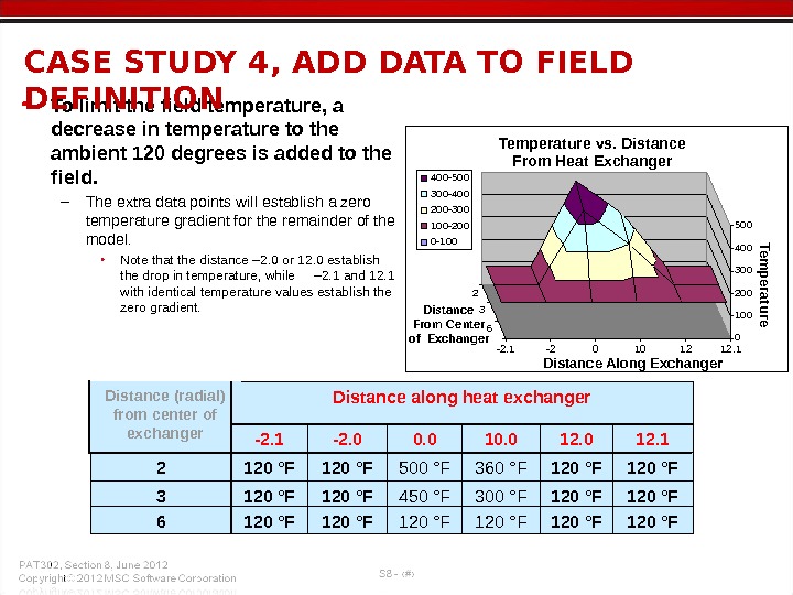
0 100 200 300 400 500 2 3 6 -2. 1 -20101212. 1 400 -500 300 -400 200 -300 100 -200 0 -100 Distance Along Exchanger. Temperature vs. Distance From Heat Exchanger. Tem perature Distance From Center of Exchanger 120 °F 300 °F 360 °F 10. 0 120 °F 12. 0 120 °F 450 °F 120 °F 3 120 °F 6 120 °F 500 °F 120 °F 2 12. 10. 0 -2. 1 Distance along heat exchanger. Distance (radial) from center of exchanger • To limit the field temperature, a decrease in temperature to the ambient 120 degrees is added to the field. – The extra data points will establish a zero temperature gradient for the remainder of the model. • Note that the distance – 2. 0 or 12. 0 establish the drop in temperature, while – 2. 1 and 12. 1 with identical temperature values establish the zero gradient. CASE STUDY 4, ADD DATA TO FIELD DEFINITION

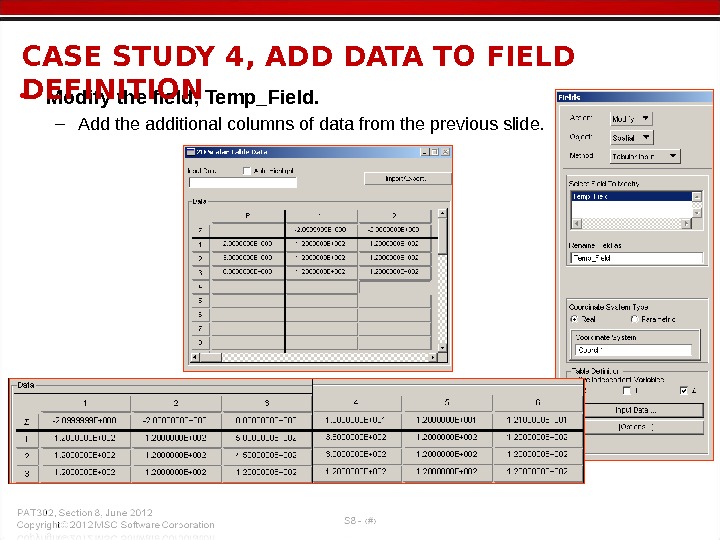
• Modify the field, Temp_Field. – Add the additional columns of data from the previous slide. CASE STUDY 4, ADD DATA TO FIELD DEFINITION

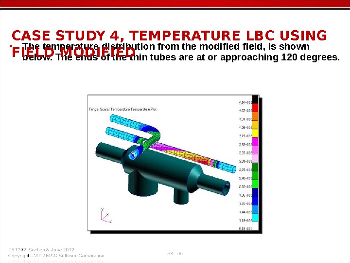
• The temperature distribution from the modified field, is shown below. The ends of the thin tubes are at or approaching 120 degrees. CASE STUDY 4, TEMPERATURE LBC USING FIELD MODIFI

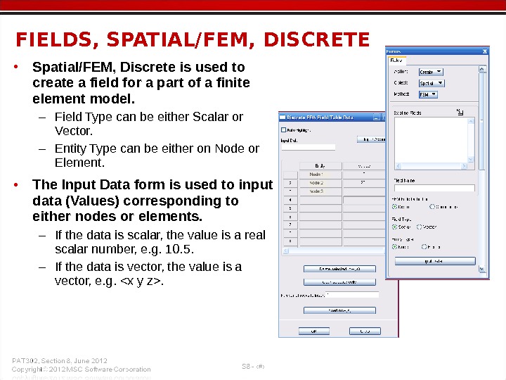
• Spatial/FEM, Discrete is used to create a field for a part of a finite element model. – Field Type can be either Scalar or Vector. – Entity Type can be either on Node or Element. • The Input Data form is used to input data (Values) corresponding to either nodes or elements. – If the data is scalar, the value is a real scalar number, e. g. 10. 5. – If the data is vector, the value is a vector, e. g. . FIELDS, SPATIAL/FEM, DISCRET

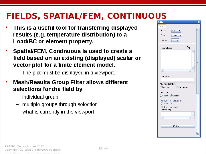
• This is a useful tool for transferring displayed results (e. g. temperature distribution) to a Load/BC or element property. • Spatial/FEM, Continuous is used to create a field based on an existing (displayed) scalar or vector plot for a finite element model. – The plot must be displayed in a viewport. • Mesh/Results Group Filter allows different selections for the field by – individual group – multiple groups through selection – what is currently in the viewport. FIELDS, SPATIAL/FEM, CONTINUOUS

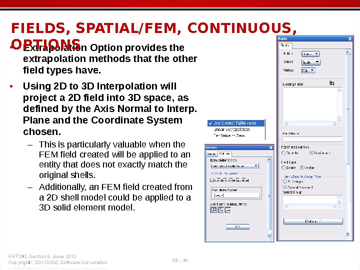
• Extrapolation Option provides the extrapolation methods that the other field types have. • Using 2 D to 3 D Interpolation will project a 2 D field into 3 D space, as defined by the Axis Normal to Interp. Plane and the Coordinate System chosen. – This is particularly valuable when the FEM field created will be applied to an entity that does not exactly match the original shells. – Additionally, an FEM field created from a 2 D shell model could be applied to a 3 D solid element model. FIELDS, SPATIAL/FEM, CONTINUOUS, OPTIONS

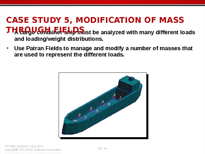
• A cargo container ship must be analyzed with many different loads and loading/weight distributions. • Use Patran Fields to manage and modify a number of masses that are used to represent the different loads. CASE STUDY 5, MODIFICATION OF MASS THROUGH FIELDS

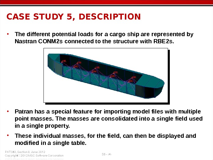
• The different potential loads for a cargo ship are represented by Nastran CONM 2 s connected to the structure with RBE 2 s. • Patran has a special feature for importing model files with multiple point masses. The masses are consolidated into a single field used in a single property. • These individual masses, for the field, can then be displayed and modified in a single table. CASE STUDY 5, DESCRIPTION

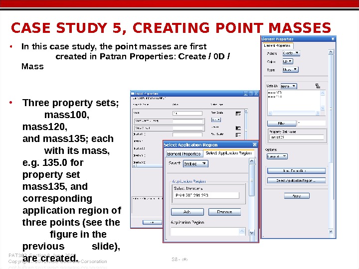
• In this case study, the point masses are first created in Patran Properties: Create / 0 D / Mass. CASE STUDY 5, CREATING POINT MASSES • Three property sets; mass 100, mass 120, and mass 135; each with its mass, e. g. 135. 0 for property set mass 135, and corresponding application region of three points (see the figure in the previous slide), are created.

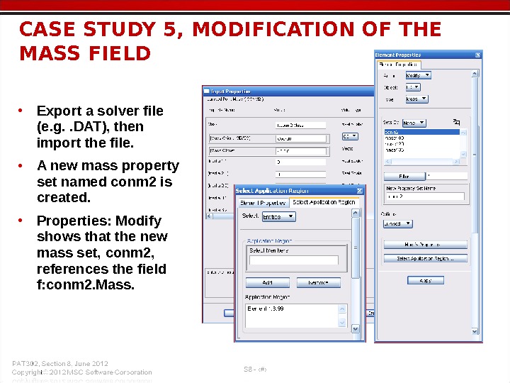
• Export a solver file (e. g. . DAT), then import the file. • A new mass property set named conm 2 is created. • Properties: Modify shows that the new mass set, conm 2, references the field f: conm 2. Mass. CASE STUDY 5, MODIFICATION OF THE MASS FIEL

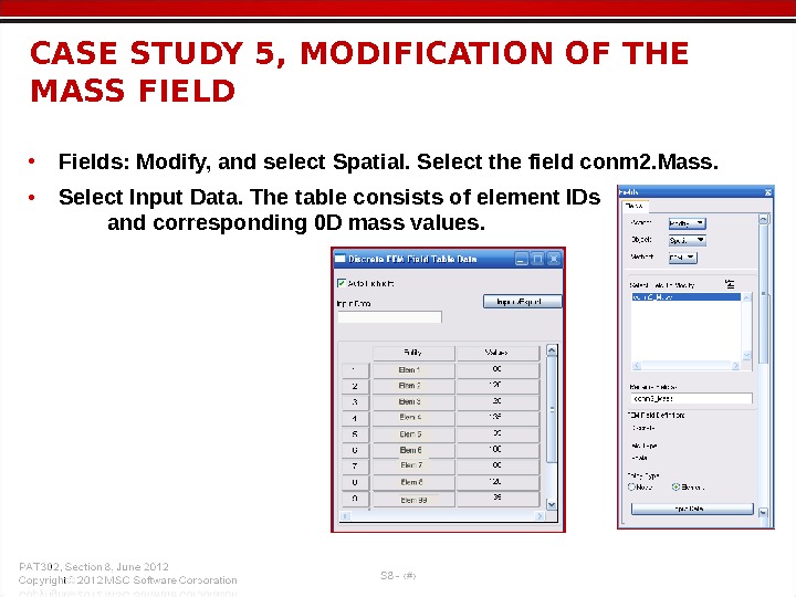
• Fields: Modify, and select Spatial. Select the field conm 2. Mass. • Select Input Data. The table consists of element IDs and corresponding 0 D mass values. CASE STUDY 5, MODIFICATION OF THE MASS FIEL

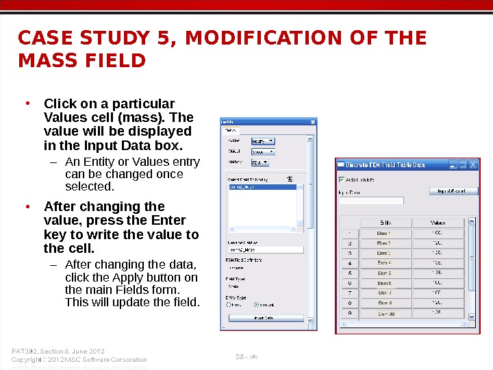
• Click on a particular Values cell (mass). The value will be displayed in the Input Data box. – An Entity or Values entry can be changed once selected. • After changing the value, press the Enter key to write the value to the cell. – After changing the data, click the Apply button on the main Fields form. This will update the field. CASE STUDY 5, MODIFICATION OF THE MASS FIEL

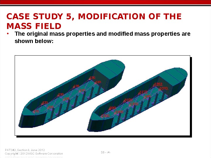
• The original mass properties and modified mass properties are shown below: CASE STUDY 5, MODIFICATION OF THE MASS FIEL

• For this case study, individual properties (e. g. mass 135, mass=135, Point 266, 291, 293) were first created, then the fields representing these properties were created as a result of exporting then importing a solver model file (e. g. . DAT). Another option would have been to make the field for the masses directly in Patran. Either approach would work. CASE STUDY 5, ALTERNATE METHO

CASE STUDY 6 FEM FIELD, CONTINUOUS CFD PRESSURE TO PATRAN PRESSUR

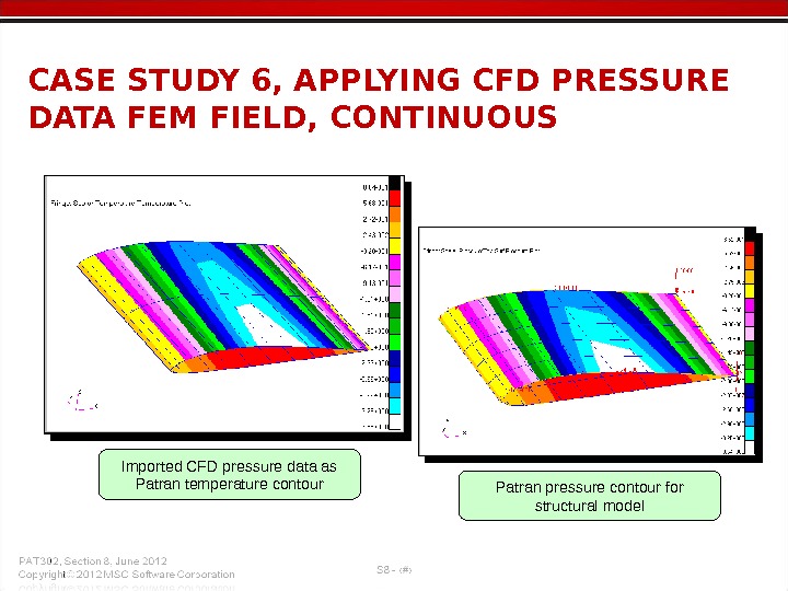
CASE STUDY 6, APPLYING CFD PRESSURE DATA FEM FIELD, CONTINUOUS Imported CFD pressure data as Patran temperature contour Patran pressure contour for structural model

• This case study demonstrates the use of FEM Field, Continuous as a way of creating an LBC for a structural model from results for a different type of model (e. g. a CFD model). • This case study demonstrates one way to get CFD pressure data into Patran. • The method shown is for CFD data in the form of point locations and corresponding pressures. • An attempt will be made to explain problems with this approach and discuss alternatives. There are other approaches for getting the data into Patran. CASE STUDY 6, FEM FIELD, CONTINUOUS

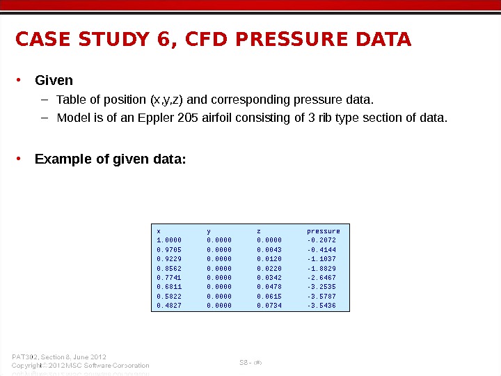
• Given – Table of position (x, y, z) and corresponding pressure data. – Model is of an Eppler 205 airfoil consisting of 3 rib type section of data. • Example of given data: CASE STUDY 6, CFD PRESSURE DATA x y z pressure 1. 0000 0. 0000 -0. 2072 0. 9705 0. 0000 0. 0043 -0. 4144 0. 9229 0. 0000 0. 0120 -1. 1037 0. 8562 0. 0000 0. 0220 -1. 8829 0. 7741 0. 0000 0. 0342 -2. 6467 0. 6811 0. 0000 0. 0478 -3. 2535 0. 5822 0. 0000 0. 0615 -3. 5787 0. 4827 0. 0000 0. 0734 -3.

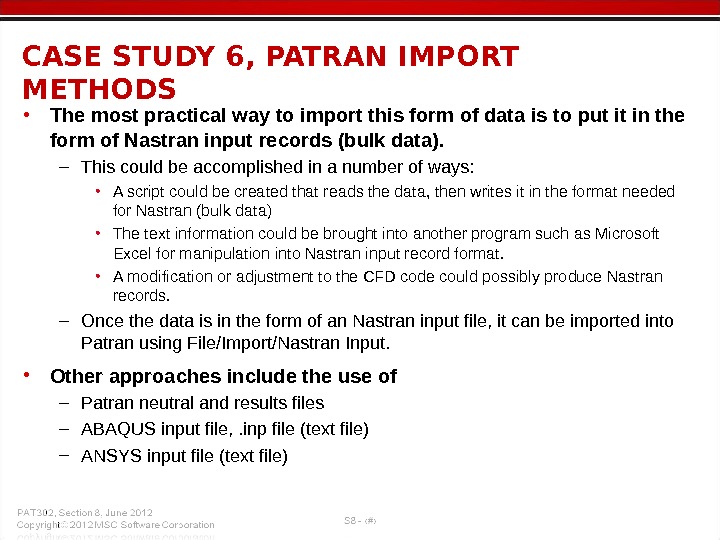
• The most practical way to import this form of data is to put it in the form of Nastran input records (bulk data). – This could be accomplished in a number of ways: • A script could be created that reads the data, then writes it in the format needed for Nastran (bulk data) • The text information could be brought into another program such as Microsoft Excel for manipulation into Nastran input record format. • A modification or adjustment to the CFD code could possibly produce Nastran records. – Once the data is in the form of an Nastran input file, it can be imported into Patran using File/Import/Nastran Input. • Other approaches include the use of – Patran neutral and results files – ABAQUS input file, . inp file (text file) – ANSYS input file (text file)CASE STUDY 6, PATRAN IMPORT METHODS

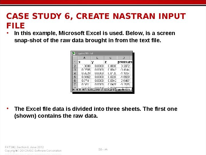
• In this example, Microsoft Excel is used. Below, is a screen snap-shot of the raw data brought in from the text file. • The Excel file data is divided into three sheets. The first one (shown) contains the raw data. CASE STUDY 6, CREATE NASTRAN INPUT FIL

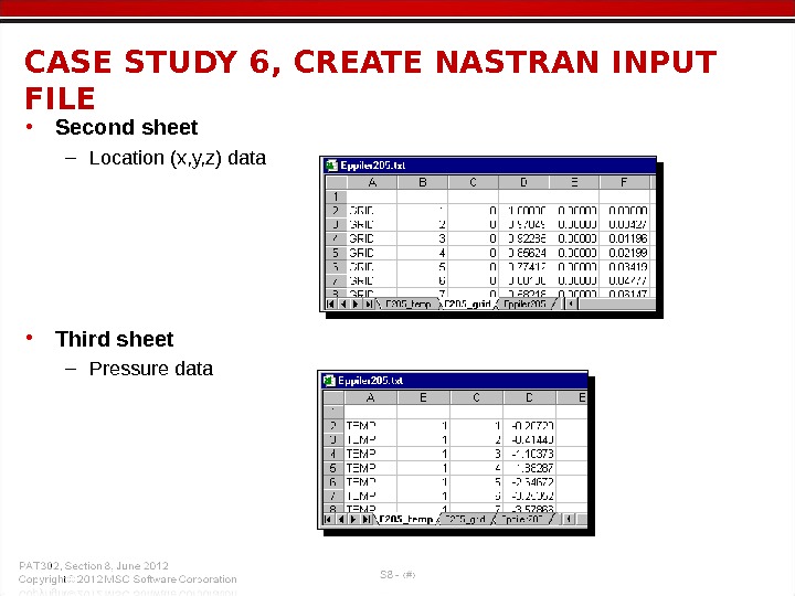
• Second sheet – Location (x, y, z) data • Third sheet – Pressure data. CASE STUDY 6, CREATE NASTRAN INPUT FIL

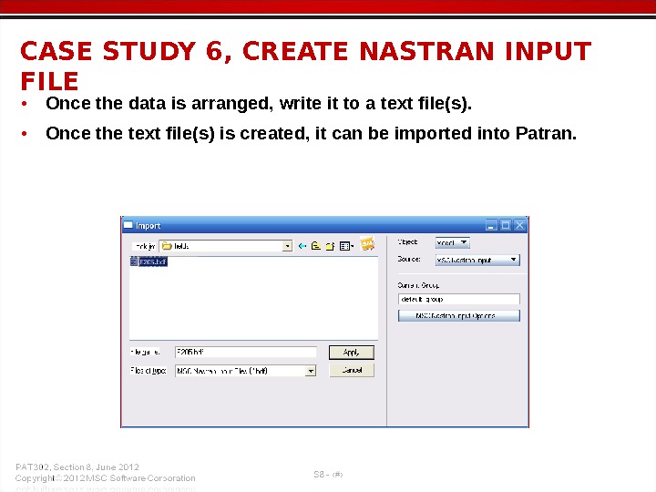
• Once the data is arranged, write it to a text file(s). • Once the text file(s) is created, it can be imported into Patran. CASE STUDY 6, CREATE NASTRAN INPUT FIL

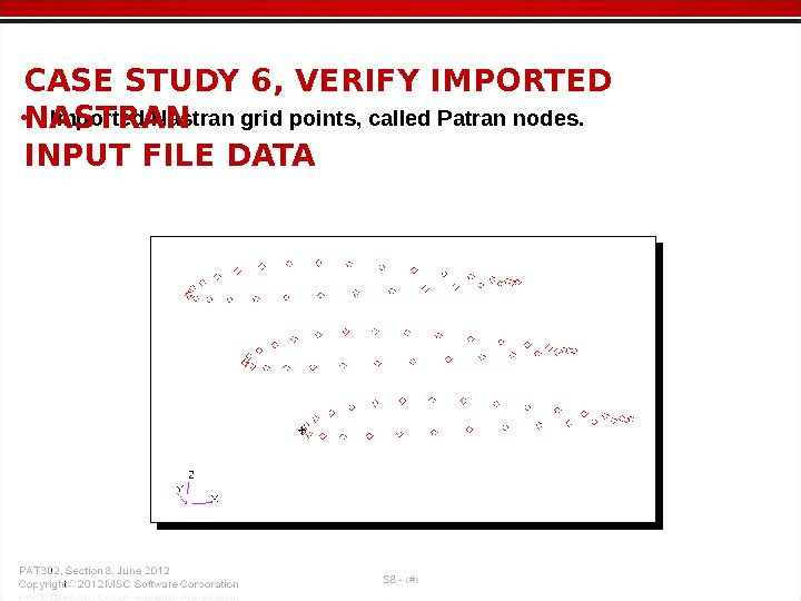
• Imported Nastran grid points, called Patran nodes. CASE STUDY 6, VERIFY IMPORTED NASTRAN INPUT FILE DAT

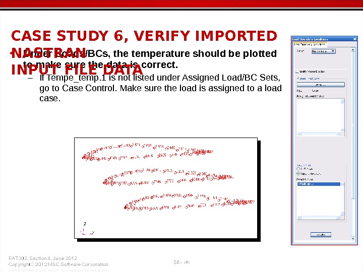
• Under Loads/BCs, the temperature should be plotted to make sure the data is correct. – If Tempe_temp. 1 is not listed under Assigned Load/BC Sets, go to Case Control. Make sure the load is assigned to a load case. CASE STUDY 6, VERIFY IMPORTED NASTRAN INPUT FILE DAT

• Use the temperature information in Patran to create pressure for a structural model. This is done using a continuous FEM Field. Once the field is created, it can then be used to create a Loads/BCs pressure set. CASE STUDY 6 TEMPERATURE TO PRESSURE IN PATRAN

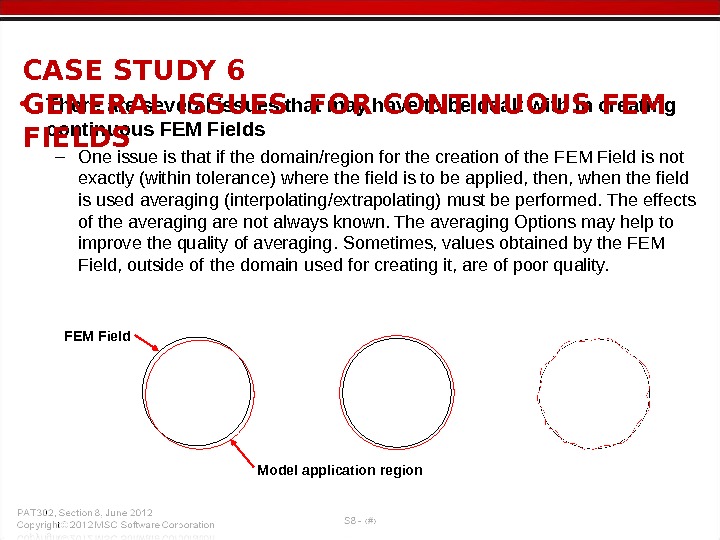
• There are several issues that may have to be dealt with in creating continuous FEM Fields – One issue is that if the domain/region for the creation of the FEM Field is not exactly (within tolerance) where the field is to be applied, then, when the field is used averaging (interpolating/extrapolating) must be performed. The effects of the averaging are not always known. The averaging Options may help to improve the quality of averaging. Sometimes, values obtained by the FEM Field, outside of the domain used for creating it, are of poor quality. CASE STUDY 6 GENERAL ISSUES FOR CONTINUOUS FEM FIELDS FEM Field Model application region

– (Continued) This issue can be partially resolved for 2 D models by enabling an Option to extend the field in one of three coordinate directions. Effectively, this maps 2 D data to 3 D space. This can be an effective method, but limits the field creation to surfaces (of elements) to those that do not overlap in that “one” direction. This can be dealt with by having a group for each surface (of elements). This is discussed herein. – Another approach is to generate the FEM Field from a domain that is slightly larger than the application region that the field will be used for. This is not always possible for the given model and data, but may be implemented in Patran by slightly scaling-up the original model. A scaling of 1% may be acceptable. – “ Secondary” FEM Field averaging is done if the model the field is being applied to is very small relative to the size of the domain used for creating the FEM Field; as the size of the model approaches the global model tolerance (e. g. 0. 005), secondary averaging is done. A possible approach for dealing with this problem is to scale-up the model, even by a factor as large as 10. CASE STUDY 6, GENERAL ISSUES FOR CONTINUOUS FEM FIELDS

– Another issue with creating FEM Fields is that this type of field must be created from a contour/fringe or vector plot that is displayed on the screen. For scalar results (e. g. temperature), only contour plots can be created, and elements are needed to create this type of plot. • This is a problem for this CASE STUDY as elements were not available with the CFD data. • Some CFD software will output elements (generally, triangular elements). If the software being used does not do this, then 2 D elements can be created manually in Patran. Sometimes, 3 D elements are necessary. CASE STUDY 6, GENERAL ISSUES FOR CONTINUOUS FEM FIELDS

• Attempts have been made to make an FEM Field with 1 D elements that connected all the grids. This FEM Field was then applied to a 2 D set of elements. The averaging was poor. The only exception was where the CFD node locations very closely or exactly coincided with the structural mesh nodes that the pressure was to be applied to. • It is not recommended to use FEM Fields created from 1 D elements unless the field is applied to 1 D elements with the same node locations. CASE STUDY 6, PROBLEM USING 1 D ELEMENTS

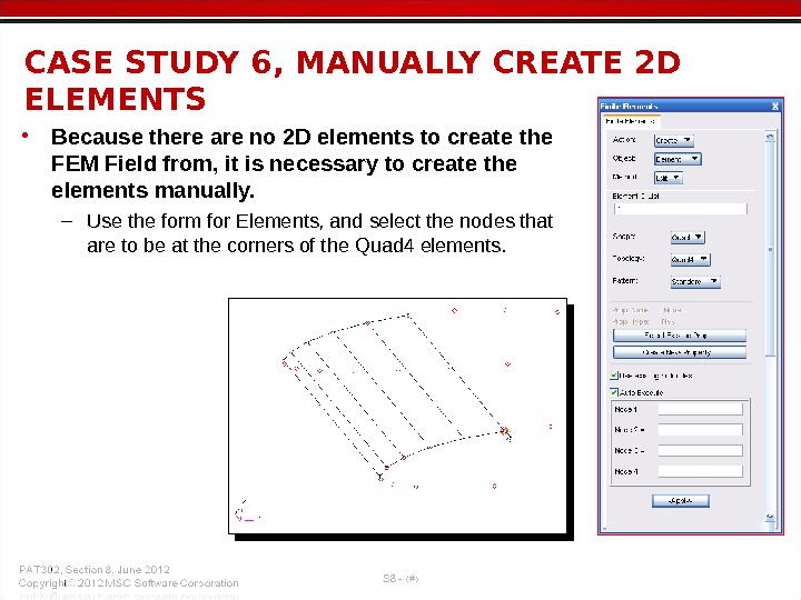
• Because there are no 2 D elements to create the FEM Field from, it is necessary to create the elements manually. – Use the form for Elements, and select the nodes that are to be at the corners of the Quad 4 elements. CASE STUDY 6, MANUALLY CREATE 2 D ELEMENTS

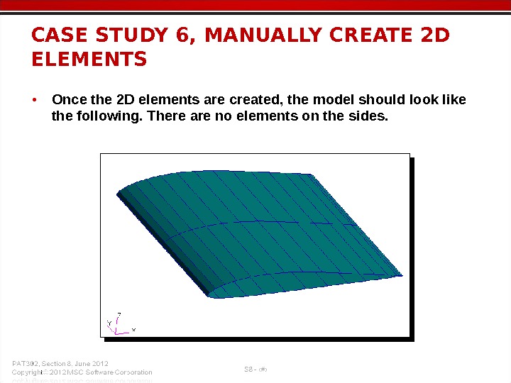
• Once the 2 D elements are created, the model should look like the following. There are no elements on the sides. CASE STUDY 6, MANUALLY CREATE 2 D ELEMENTS

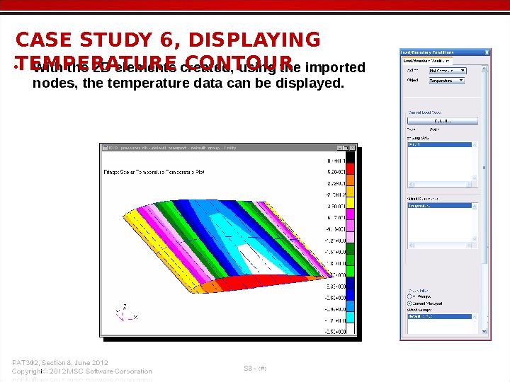
• With the 2 D elements created, using the imported nodes, the temperature data can be displayed. CASE STUDY 6, DISPLAYING TEMPERATURE CONTOUR

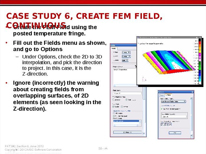
• Create the FEM Field using the posted temperature fringe. • Fill out the Fields menu as shown, and go to Options – Under Options, check the 2 D to 3 D interpolation, and pick the direction to project. In this case, it is the Z-direction. • Ignore (incorrectly) the warning about creating fields from overlapping surfaces, of 2 D elements (as seen looking in the Z-direction). CASE STUDY 6, CREATE FEM FIELD, CONTINUOUS

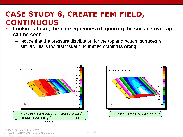
• Looking ahead, the consequences of ignoring the surface overlap can be seen. – Notice that the pressure distribution for the top and bottom surfaces is similar. This is the first visual clue that something is wrong. CASE STUDY 6, CREATE FEM FIELD, CONTINUOUS Field, and subsequently, pressure LBC made incorrectly from a temperature contour. Original Temperature Contour

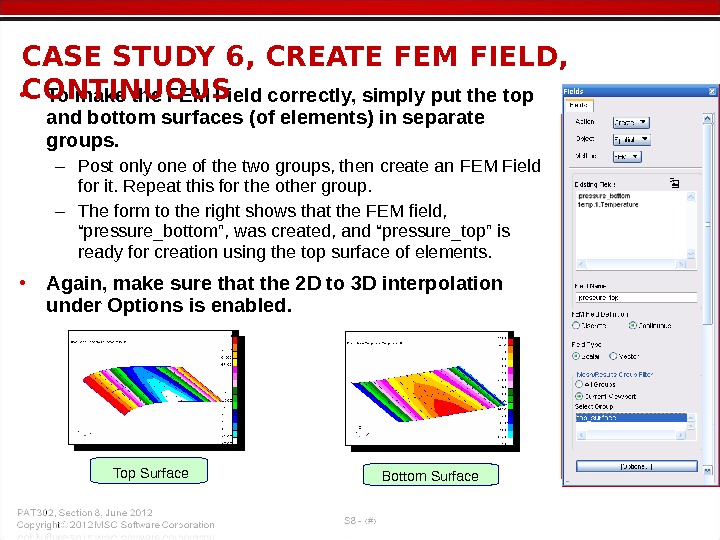
• To make the FEM Field correctly, simply put the top and bottom surfaces (of elements) in separate groups. – Post only one of the two groups, then create an FEM Field for it. Repeat this for the other group. – The form to the right shows that the FEM field, “pressure_bottom”, was created, and “pressure_top” is ready for creation using the top surface of elements. • Again, make sure that the 2 D to 3 D interpolation under Options is enabled. CASE STUDY 6, CREATE FEM FIELD, CONTINUOUS Bottom Surface. Top Surface

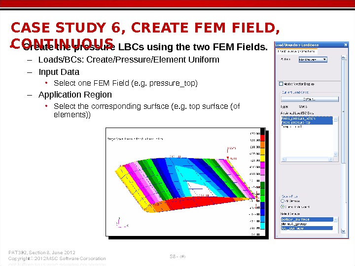
• Create the pressure LBCs using the two FEM Fields. – Loads/BCs: Create/Pressure/Element Uniform – Input Data • Select one FEM Field (e. g. pressure_top) – Application Region • Select the corresponding surface (e. g. top surface (of elements))CASE STUDY 6, CREATE FEM FIELD, CONTINUOUS

• Perform Workshop 19 “Global/Local Modeling Using FEM Fields” in your exercise workbook. EXERCISES

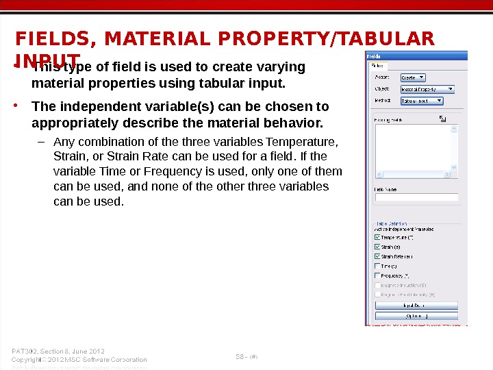
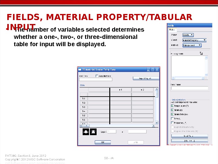
• This type of field is used to create varying material properties using tabular input. • The independent variable(s) can be chosen to appropriately describe the material behavior. – Any combination of the three variables Temperature, Strain, or Strain Rate can be used for a field. If the variable Time or Frequency is used, only one of them can be used, and none of the other three variables can be used. FIELDS, MATERIAL PROPERTY/TABULAR INPUT

• The number of variables selected determines whether a one , two , or three dimensional ‑ ‑ ‑ table for input will be displayed. FIELDS, MATERIAL PROPERTY/TABULAR INPUT

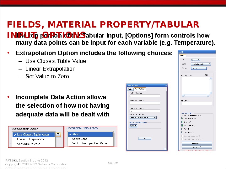
• The top portion of the Tabular Input, [Options] form controls how many data points can be input for each variable (e. g. Temperature). • Extrapolation Option includes the following choices: – Use Closest Table Value – Linear Extrapolation – Set Value to Zero • Incomplete Data Action allows the selection of how not having adequate data will be dealt with. FIELDS, MATERIAL PROPERTY/TABULAR INPUT, OPTIONS

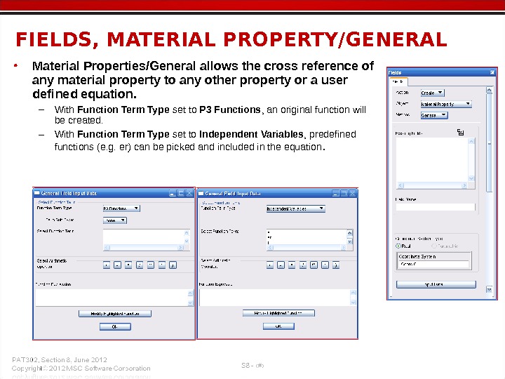
• Material Properties/General allows the cross reference of any material property to any other property or a user defined equation. – With Function Term Type set to P 3 Functions , an original function will be created. – With Function Term Type set to Independent Variables , predefined functions (e. g. er) can be picked and included in the equation. FIELDS, MATERIAL PROPERTY/GENERAL

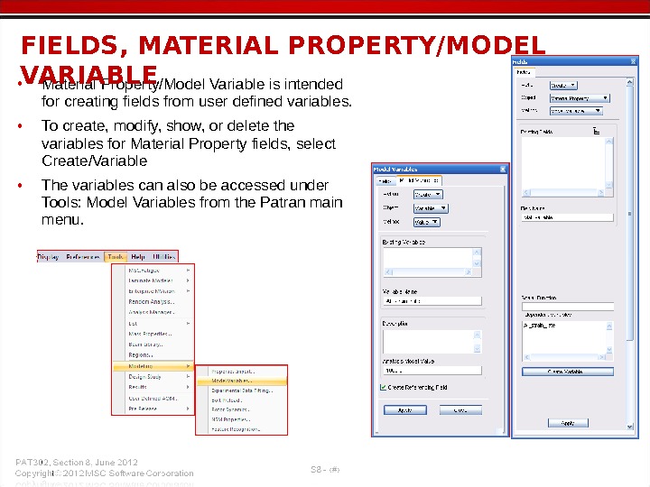
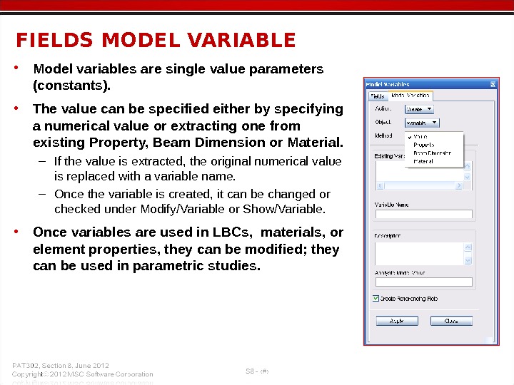
• Material Property/Model Variable is intended for creating fields from user defined variables. • To create, modify, show, or delete the variables for Material Property fields, select Create/Variable • The variables can also be accessed under Tools: Model Variables from the Patran main menu. FIELDS, MATERIAL PROPERTY/MODEL VARIABL

• Model variables are single value parameters (constants). • The value can be specified either by specifying a numerical value or extracting one from existing Property, Beam Dimension or Material. – If the value is extracted, the original numerical value is replaced with a variable name. – Once the variable is created, it can be changed or checked under Modify/Variable or Show/Variable. • Once variables are used in LBCs, materials, or element properties, they can be modified; they can be used in parametric studies. FIELDS MODEL VARIABL

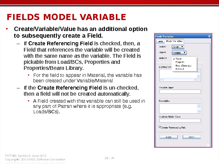
• Create/Variable/Value has an additional option to subsequently create a Field. – If Create Referencing Field is checked, then, a Field that references the variable will be created with the same name as the variable. The Field is pickable from Load/BCs, Properties and Properties/Beam Library. • For the field to appear in Material, the variable has been created under Variable/Material – If the Create Referencing Field is un-checked, then a field will not be created automatically. • A Field created with that variable can still be used in any part of Patran where it is appropriate (e. g. Loads/BCs). FIELDS MODEL VARIABL

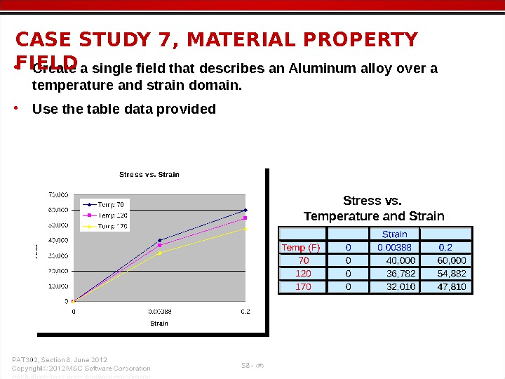
Stress vs. Temperature and Strain • Create a single field that describes an Aluminum alloy over a temperature and strain domain. • Use the table data provided. CASE STUDY 7, MATERIAL PROPERTY FIEL

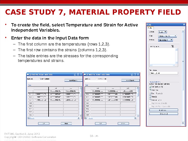
CASE STUDY 7, MATERIAL PROPERTY FIELD • To create the field, select Temperature and Strain for Active Independent Variables. • Enter the data in the Input Data form – The first column are the temperatures (rows 1, 2, 3). – The first row contains the strains (columns 1, 2, 3). – The table entries are the stresses for the corresponding temperatures and strains.

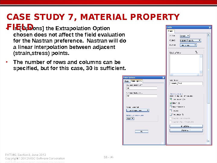
• In [Options] the Extrapolation Option chosen does not affect the field evaluation for the Nastran preference. Nastran will do a linear interpolation between adjacent (strain, stress) points. • The number of rows and columns can be specified, but for this case, 30 is sufficient. CASE STUDY 7, MATERIAL PROPERTY FIEL

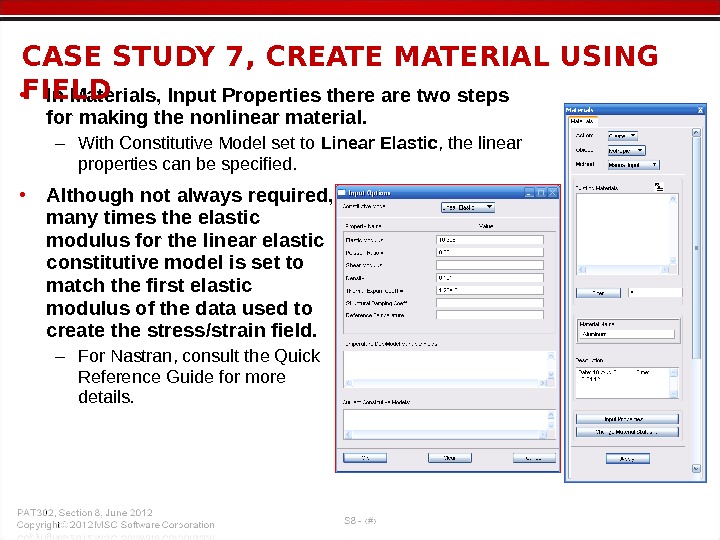
• In Materials, Input Properties there are two steps for making the nonlinear material. – With Constitutive Model set to Linear Elastic , the linear properties can be specified. • Although not always required, many times the elastic modulus for the linear elastic constitutive model is set to match the first elastic modulus of the data used to create the stress/strain field. – For Nastran, consult the Quick Reference Guide for more details. CASE STUDY 7, CREATE MATERIAL USING FIEL

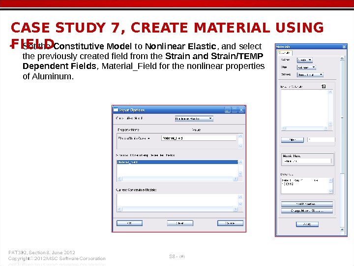
• Set the Constitutive Model to Nonlinear Elastic , and select the previously created field from the Strain and Strain/TEMP Dependent Fields , Material_Field for the nonlinear properties of Aluminum. CASE STUDY 7, CREATE MATERIAL USING FIEL

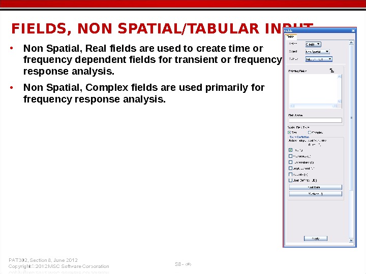
• Non Spatial, Real fields are used to create time or frequency dependent fields for transient or frequency response analysis. • Non Spatial, Complex fields are used primarily for frequency response analysis. FIELDS, NON SPATIAL/TABULAR INPUT

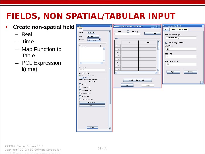
• Create non-spatial field – Real – Time – Map Function to Table – PCL Expression f(time)FIELDS, NON SPATIAL/TABULAR INPUT

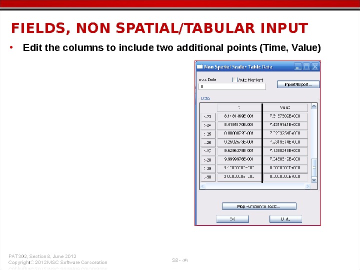
• Edit the columns to include two additional points (Time, Value)FIELDS, NON SPATIAL/TABULAR INPUT

FIELDS, NON SPATIAL/TABULAR INPUT

FIELDS, NON SPATIAL/TABULAR INPUT