Merge_sort.pptx
- Количество слайдов: 26


![Recursive binary search int r. Binary. Search(int sorted. Array[], int first, int last, int](https://present5.com/presentation/133062010_139920382/image-1.jpg "Recursive binary search int r. Binary. Search(int sorted. Array[], int first, int last, int")
Recursive binary search int r. Binary. Search(int sorted. Array[], int first, int last, int key) { if (first <= last) { int mid = (first + last) / 2; // compute mid point. if (key == sorted. Array[mid]) return mid; // found it. else if (key < sorted. Array[mid]) // Call ourself for the lower part of the array return r. Binary. Search(sorted. Array, first, mid-1, key); else // Call ourself for the upper part of the array return r. Binary. Search(sorted. Array, mid+1, last, key); } return -(first + 1); // failed to find key }

Merge sort

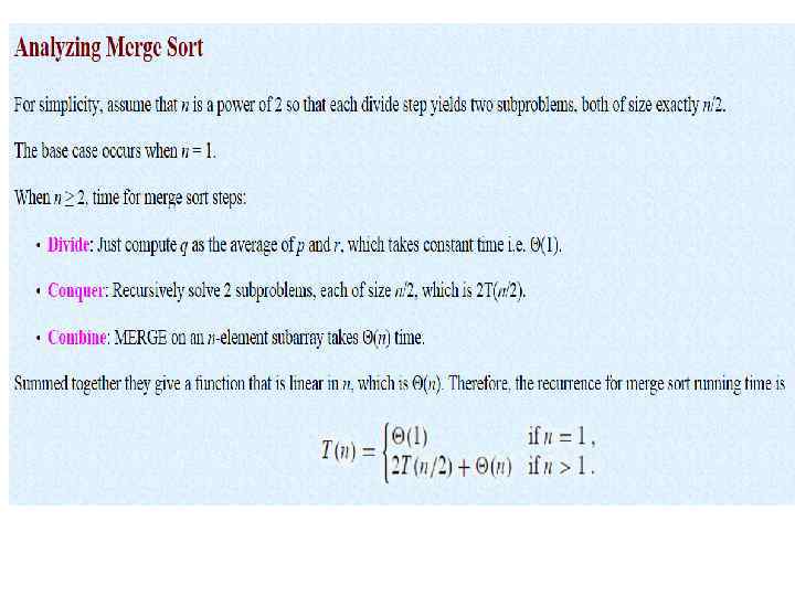
• Merge sort is based on the divide-andconquer paradigm. Its worst-case running time has a lower order of growth than insertion sort. Since we are dealing with subproblems, we state each subproblem as sorting a subarray A[p. . r]. Initially, p = 1 and r = n, but these values change as we recurse through subproblems.
![To sort A[p. . r]: • 1. Divide Step If a given array A](https://present5.com/presentation/133062010_139920382/image-4.jpg "To sort A[p. . r]: • 1. Divide Step If a given array A")
To sort A[p. . r]: • 1. Divide Step If a given array A has zero or one element, simply return; it is already sorted. Otherwise, split A[p. . r] into two subarrays. A[p. . q] and A[q + 1. . r], each containing about half of the elements of A[p. . r]. That is, q is the halfway point of A[p. . r]. • 2. Conquer Step Conquer by recursively sorting the two subarrays A[p. . q] and A[q + 1. . r]. • 3. Combine Step Combine the elements back in A[p. . r] by merging the two sorted subarrays. A[p. . q] and A[q + 1. . r] into a sorted sequence. To accomplish this step, we will define a procedure MERGE (A, p, q, r). Note that the recursion bottoms out when the subarray has just one element, so that it is trivially sorted.
![Algorithm: Merge Sort To sort the entire sequence A[1. . n], make the initial](https://present5.com/presentation/133062010_139920382/image-5.jpg "Algorithm: Merge Sort To sort the entire sequence A[1. . n], make the initial")
Algorithm: Merge Sort To sort the entire sequence A[1. . n], make the initial call to the procedure MERGE-SORT (A, 1, n). MERGE-SORT (A, p, r) 1. IF p < r // Check for base case 2. THEN q = FLOOR[(p +r)/2] // Divide step 3. MERGE_SORT (A, p, q) // Conquer step. 4. MERGE_SORT (A, q + 1, r) // Conquer step. 5. MERGE (A, p, q, r) // Conquer step.

Example: Bottom-up view of the above procedure for n = 8.

Merging What remains is the MERGE procedure. The following is the input and output of the MERGE procedure. • INPUT: Array A and indices p, q, r such that p ≤ q ≤ r and subarray. A[p. . q] is sorted and subarray A[q + 1. . r] is sorted. By restrictions onp, q, r, neither subarray is empty. • OUTPUT: The two subarrays are merged into a single sorted subarray in A[p. . r]. We implement it so that it takes Θ(n) time, where n = r − p + 1, which is the number of elements being merged.

The pseudocode of the MERGE procedure is as follow:

Running Time The first two for loops (that is, the loop in line 4 and the loop in line 6) take Θ(n 1 + n 2) =Θ(n) time. The last for loop (that is, the loop in line 12) makes n iterations, each taking constant time, for Θ(n) time. Therefore, the total running time is Θ(n).

Recursion Tree We can understand how to solve the merge-sort recurrence without the master theorem. There is a drawing of recursion tree on page 35 in CLRS, which shows successive expansions of the recurrence. The following figure (Figure 2. 5 b in CLRS) shows that for the original problem, we have a cost of cn, plus the two subproblems, each costing T (n/2).

The following figure tells to continue expanding until the problem sizes get down to 1.

• In the above recursion tree, each level has cost cn. • The top level has cost cn. • The next level down has 2 subproblems, each contributing cost cn/2. • The next level has 4 subproblems, each contributing cost cn/4. • Each time we go down one level, the number of subproblems doubles but the cost per subproblem halves. Therefore, cost per level stays the same. • The height of this recursion tree is lg n and there are lg n + 1 levels.
![Implementation void merge_sort(int a[], int temp[], int size){ m_sort(a, temp, 0, size-1); }](https://present5.com/presentation/133062010_139920382/image-14.jpg "Implementation void merge_sort(int a[], int temp[], int size){ m_sort(a, temp, 0, size-1); }")
Implementation void merge_sort(int a[], int temp[], int size){ m_sort(a, temp, 0, size-1); }
![void m_sort(int a[], int temp[], int left, int right){ int mid; if(right>left){ mid =](https://present5.com/presentation/133062010_139920382/image-15.jpg "void m_sort(int a[], int temp[], int left, int right){ int mid; if(right>left){ mid =")
void m_sort(int a[], int temp[], int left, int right){ int mid; if(right>left){ mid = (right+left)/2; m_sort(a, temp, left, mid); m_sort(a, temp, mid+1, right); merge(a, temp, left, mid+1, right); } }
![void merge(int a[], int temp[], int left, int mid, int right){ int i, left_end,](https://present5.com/presentation/133062010_139920382/image-16.jpg "void merge(int a[], int temp[], int left, int mid, int right){ int i, left_end,")
void merge(int a[], int temp[], int left, int mid, int right){ int i, left_end, num_elements, tmp_pos; left_end = mid - 1; tmp_pos = left; num_elements = right - left +1; while((left<=left_end) && (mid<=right)) { if(a[left]<=a[mid]) { temp[tmp_pos] = a[left]; tmp_pos = tmp_pos+1; left = left+1; } else{ temp[tmp_pos]=a[mid]; tmp_pos = tmp_pos+1; mid = mid+1; } }
![while(left<=left_end){ temp[tmp_pos] = a[left]; left = left+1; tmp_pos++; } while(mid<=right){ temp[tmp_pos] = a[mid]; mid++;](https://present5.com/presentation/133062010_139920382/image-17.jpg "while(left<=left_end){ temp[tmp_pos] = a[left]; left = left+1; tmp_pos++; } while(mid<=right){ temp[tmp_pos] = a[mid]; mid++;")
while(left<=left_end){ temp[tmp_pos] = a[left]; left = left+1; tmp_pos++; } while(mid<=right){ temp[tmp_pos] = a[mid]; mid++; tmp_pos++; } for(i=0; i<=num_elements; i++) { a[right] = temp[right]; right = right - 1; } }
![• int main(){ • int a[10] = {1, 5, 0, 2, 4, 7,](https://present5.com/presentation/133062010_139920382/image-18.jpg "• int main(){ • int a[10] = {1, 5, 0, 2, 4, 7,")
• int main(){ • int a[10] = {1, 5, 0, 2, 4, 7, 8}; • int temp[10]; • merge_sort(a, temp, 10); • for(int i=0; i<10; i++) • cout<<a[i]<<endl; • system("pause"); • return 0; • }

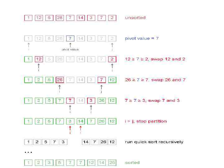
Quick sort Quicksort is a fast sorting algorithm, which is used not only for educational purposes, but widely applied in practice. On the average, it has O(n log n) complexity, making quicksort suitable for sorting big data volumes. The idea of the algorithm is quite simple and once you realize it, you can write quicksort as fast as bubble sort. Algorithm • The divide-and-conquer strategy is used in quicksort. Below the recursion step is described: 1. Choose a pivot value. We take the value of the middle element as pivot value, but it can be any value, which is in range of sorted values, even if it doesn't present in the array. 2. Partition. Rearrange elements in such a way, that all elements which are lesser than the pivot go to the left part of the array and all elements greater than the pivot, go to the right part of the array. Values equal to the pivot can stay in any part of the array. Notice, that array may be divided in non-equal parts. 3. Sort both parts. Apply quicksort algorithm recursively to the left and the right parts. •

Partition algorithm in detail There are two indices i and j and at the very beginning of the partition algorithm i points to the first element in the array and j points to the last one. Then algorithm moves i forward, until an element with value greater or equal to the pivot is found. Index j is moved backward, until an element with value lesser or equal to the pivot is found. If i ≤ j then they are swapped and i steps to the next position (i + 1), j steps to the previous one (j - 1). Algorithm stops, when i becomes greater than j. After partition, all values before i-th element are less or equal than the pivot and all values after j-th element are greater or equal to the pivot.
 complexity, but strong")
Complexity analysis • On the average quicksort has O(n log n) complexity, but strong proof of this fact is not trivial and not presented here. In worst case, quicksort runs O(n 2) time, but on the most "practical" data it works just fine and outperforms other O(n log n) sorting algorithms.

Best Case The best thing that could happen in Quick sort would be that each partitioning stage divides the array exactly in half. In other words, the best to be a median of the keys in A[p. . r] every time procedure 'Partition' is called. The procedure 'Partition' always split the array to be sorted into two equal sized arrays. If the procedure 'Partition' produces two regions of size n/2. the recurrence relation is then
![Worst case Partitioning The worst-case occurs if given array A[1. . n] is already](https://present5.com/presentation/133062010_139920382/image-24.jpg "Worst case Partitioning The worst-case occurs if given array A[1. . n] is already")
Worst case Partitioning The worst-case occurs if given array A[1. . n] is already sorted. The PARTITION (A, p, r) call always return p so successive calls to partition will split arrays of length n, n-1, n-2, . . . , 2 and running time proportional to n + (n-1) + (n-2) +. . . + 2 = [(n+2)(n-1)]/2 = (n 2). The worst-case also occurs if A[1. . n] starts out in reverse order.
![Implementation 4 3 2 3 5 8 7 5 void quick. Sort(int arr[], int](https://present5.com/presentation/133062010_139920382/image-25.jpg "Implementation 4 3 2 3 5 8 7 5 void quick. Sort(int arr[], int")
Implementation 4 3 2 3 5 8 7 5 void quick. Sort(int arr[], int left, int right) { int i = left, j = right; int tmp; int pivot = arr[(left + right) / 2]; /* partition */ while (i <= j) { while (arr[i] < pivot) i++; while (arr[j] > pivot) j--; if (i <= j) { tmp = arr[i]; arr[i] = arr[j]; arr[j] = tmp; i++; j--; } };
 quick. Sort(arr, left, j); if (i <")
/* recursion */ if (left < j) quick. Sort(arr, left, j); if (i < right) quick. Sort(arr, i, right); }
Merge_sort.pptx